# PDI to Jupyter Notebook

{% hint style="warning" %}

#### **Workshop - PDI to Jupyter Notebook**

This workshop demonstrates how to create a Pentaho Data Integration (PDI) pipeline that processes sales data and automatically triggers analysis in Jupyter Notebook when the output file is saved.

The topics were going to cover:

* Creating a Jupyter Notebook
* Installing required Python packages: `jupyter`, `watchdog`, `xslxwriter`
* Create a PDI pipeline: sales\_data.csv file
* Create a File Watcher script
  {% endhint %}

<figure><img src="/files/Et4PZ08PY5A3CQP8MzUU" alt=""><figcaption><p>Pipeline</p></figcaption></figure>

{% hint style="info" %}
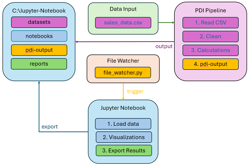
Quick overview of the pipeline:

* Execute a PDI pipeline with sample sales\_data.csv - from datasets folder
* The file output to the pdi-output folder triggers the Jupyter Notebook to
* Load the data - csv files from pdi-output - analyze and visualize the results
* Export the results to the reports folder
  {% endhint %}

***

{% hint style="info" %}
**Create a new Transformation**

Any one of these actions opens a new Transformation tab for you to begin designing your transformation.

* By clicking File > New > Transformation
* By using the CTRL-N hot key
  {% endhint %}

Select the Host Docker OS:

{% tabs %}
{% tab title="Linux" %}
{% hint style="info" %}

#### PDI to Jupyter Notebook

{% endhint %}

{% tabs %}
{% tab title="1. Setup Verification" %}
{% hint style="info" %}

#### Setup Verification

Before building the PDI pipeline, verify everything works by running the sample notebook.
{% endhint %}

1. Verify Python Packages are Installed.

```bash
# Check that packages were auto-installed
docker exec jupyter-datascience pip list | grep -E "watchdog|xlsxwriter"
# Expected: watchdog x.x.x  and  XlsxWriter x.x.x
```

{% hint style="info" %}
Python packages (`watchdog`, `xlsxwriter`) are **automatically installed** when the container starts via the `post-start.sh` startup script.

If packages are missing, check the container logs: `docker logs jupyter-datascienc`
{% endhint %}

2. Verify Test Files Exist (Inside the Container).

```bash
# Still inside the container shell:
docker exec -it jupyter-datascience sh

# Check for datasets
cd /home/jovyan/datasets
ls
# Expected: orders.csv  sales_data.csv

# Check for notebooks
cd /home/jovyan/notebooks
ls
# Expected: sales_analysis.ipynb  welcome.ipynb

# Exit the container shell
exit
```

***

**Run the Sales Analysis Notebook**

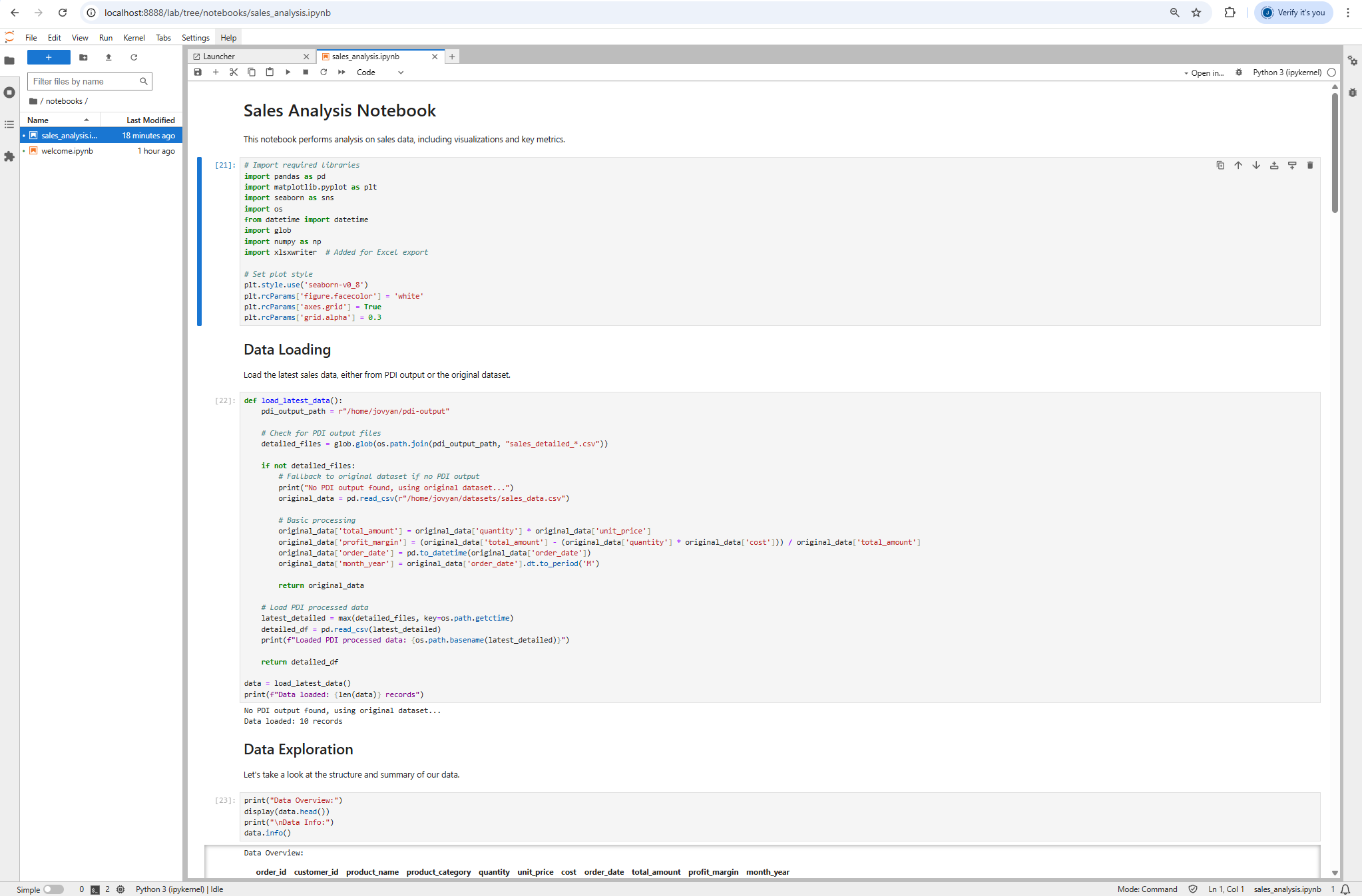
1. In Jupyter Lab, navigate to **notebooks/** in the file browser
2. Open **sales\_analysis.ipynb**
3. Run each cell in order (Shift+Enter or use the Run menu)
4. The notebook will:
   * Load `sales_data.csv` from `/home/jovyan/datasets/`
   * Generate a 4-panel Sales Analysis Dashboard
   * Calculate Key Metrics (revenue, average order value, profit margin)
   * Export an Excel report to `/home/jovyan/reports/`

<figure><img src="/files/wNRRCM2gOzUig6PfPMKy" alt=""><figcaption><p>sales_analysis.ipynb</p></figcaption></figure>

5. Check the Output Report

```bash
# On the host machine, check for the generated report
ls ~/Jupyter-Notebook/reports/
# Expected: sales_analysis_<timestamp>.xlsx
```

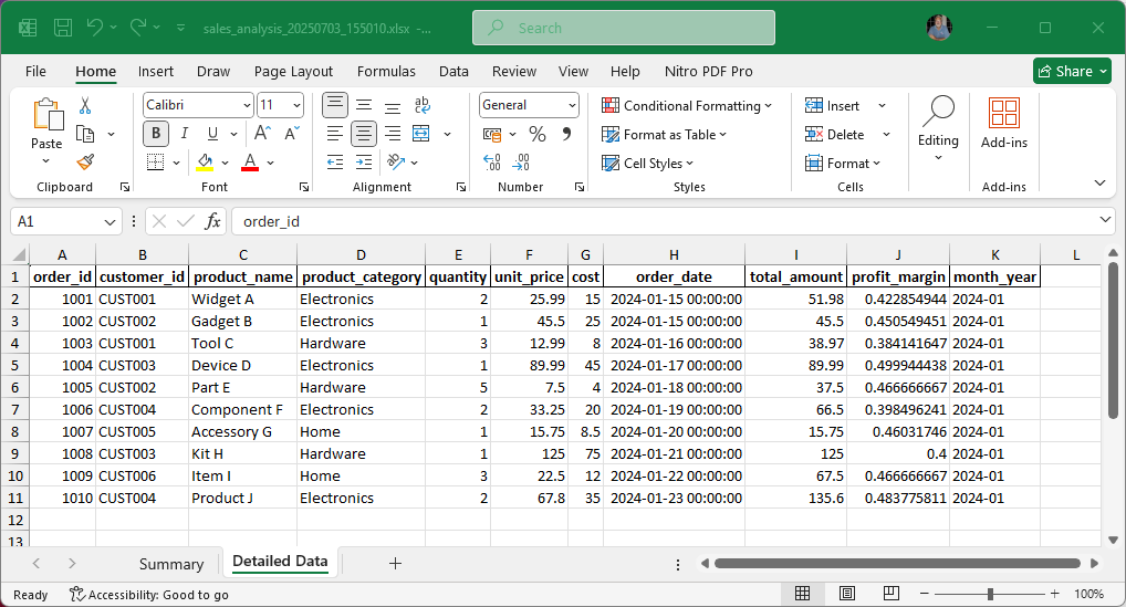
Open the Excel file and verify it has two sheets:

* **Summary** - Key metrics (Total Revenue, Average Order Value, etc.)
* **Detailed Data** - Full processed dataset

<figure><img src="/files/4JBspnYq14DVoZl1aDC7" alt=""><figcaption><p>sales_analysis</p></figcaption></figure>
{% endtab %}

{% tab title="2. PDI pipeline" %}
{% hint style="info" %}

#### Build the PDI Pipeline

The data scientists have deployed the sales\_analysis.ipynb notebook. The notebook will be triggered by a File Watcher that's polling the \~/Jupyter-Notebook/pdi-output/ for:

* sales\_detailed\_\*.csv

So in this part of the workshop, we're going to create a simple pipeline that:

* Loads the sales.csv
* Cleans and performs some calculations and aggregations
* Outputs to: \~/Jupyter-Notebook/pdi-output/ folder.
  {% endhint %}

1. Start Pentaho Data Integration (Spoon)

```bash
# Navigate to the PDI installation
cd
cd ~/Pentaho/design-tools/data-integration

# Launch Spoon (the PDI graphical designer)
./spoon.sh
```

2. Create a New Transformation - sales\_pipeline.ktr:

<figure><img src="/files/wc4yXOVvhmStK31dnZJa" alt=""><figcaption><p>sales_pipeline.ktr</p></figcaption></figure>

{% file src="/files/WmBEitG9qAyyARlGxF7q" %}

{% file src="/files/0MzlYl8FsUkRYq0f4K9F" %}

{% tabs %}
{% tab title="1. CSV File input" %}
{% hint style="info" %}

#### **CSV File input**

The CSV File Input transform extracts data from delimited files using either a predefined schema or manually configured field layouts. Despite its name, this transform supports any delimiter—pipes, tabs, semicolons, or custom separators—not just commas.

Built for speed through optimized internal processing, this transform offers a focused subset of Text File Input capabilities with three key performance advantages:

**Native I/O (NIO)** uses direct system calls for faster file reading, though it's currently limited to local files without VFS support.

**Parallel Processing** enables distributed file reading when running multiple transform copies or in clustered mode. Each copy processes a separate file block, allowing workload distribution across multiple threads or slave nodes.

**Lazy Conversion** optimizes performance for pass-through data scenarios. When fields flow unchanged from input to output (like file-to-database transfers), this feature prevents unnecessary data type conversions, avoiding the overhead of converting raw data into strings, dates, or numbers.

While this transform has fewer configuration options than the general Text File Input transform, these performance optimizations make it ideal for high-throughput data processing workflows.
{% endhint %}

1. Drag & drop a CSV File input step onto the canvas.
2. Double-click on the step, and configure the following properties:

<figure><img src="/files/HZkBxXDkqUnEG6PGqOVs" alt=""><figcaption><p>CSV file input</p></figcaption></figure>

**CSV File Input**

* **Step type:** Input > CSV file input
* **Purpose:** Reads the source sales data
* **Configuration:**
  1. Drag a **CSV file input** step onto the canvas
  2. Double-click to configure:
     * **Filename:** `~/Jupyter-Notebook/datasets/sales_data.csv`
     * **Delimiter:** `,`
     * **Header row present:** checked
  3. Click **Get Fields** to auto-detect the 8 columns
  4. Verify the field types: `order_id` (Integer), `customer_id` (Integer), `product_name` (String), `product_category` (String), `quantity` (Integer), `unit_price` (Number), `cost` (Number), `order_date` (String)
  5. Click **Preview** to verify data loads correctly (should show 250 rows)
     {% endtab %}

{% tab title="2. Data Validator" %}
{% hint style="info" %}

#### **Data Validator**

The Data Validator transform enables you to define validation rules that check input data across different fields in each row. When the validator encounters a row that violates one or more validation rules, it generates an error or exception.

You can capture all validation errors by configuring an error handling hop from this transform, which will provide you with a comprehensive list of any validation failures that occur during processing.
{% endhint %}

1. Drag & drop Data Validator step onto the canvas.
2. Double-click on the step, and configure the following properties:

**Validation: quantity**

<figure><img src="/files/3KXKZklsMiwMGtZjtxZm" alt=""><figcaption><p>Validation - quantity</p></figcaption></figure>

**Validation: unit\_price**

<figure><img src="/files/XQzzpBYuf0UgkW0Ft1Zm" alt=""><figcaption><p>Validation - unit_price</p></figcaption></figure>

**Data Validator (optional)**

* **Step type:** Validation > Data Validator
* **Purpose:** Validates input data quality
* **Configuration:**
  1. Add a **Data Validator** step and connect it from CSV file input
  2. Add validations:
     * `quantity`: Data type = Integer, Minimum value = 1
     * `unit_price`: Data type = BigNumber, Minimum value = 0.01
  3. Create an **error handling hop** (red hop) to a **Dummy** step for invalid records
     {% endtab %}

{% tab title="3. Replace in String" %}
{% hint style="info" %}

#### **Replace in String**

The Replace In String transform performs simple search and replace operations on String fields.

It also supports regular expressions and group references. group references are picked up in the replace by string as $n where n is the number of the group.

You can also use hexadecimal replacements for special characters.
{% endhint %}

1. Drag & drop Replace in string step onto the canvas.
2. Double-click on the step, and configure the following properties:

<figure><img src="/files/wItI76AoVWprdCMhYUat" alt=""><figcaption><p>Replace in string - standardize</p></figcaption></figure>

**Replace in String**

* **Step type:** Transform > Replace in String
* **Purpose:** Normalise the inconsistent `product_category` casing
* **Configuration:**
  1. Add a **Replace in String** step
  2. Add rows to fix each category (the dataset has mixed case like `electronics` / `Electronics`):

     <table><thead><tr><th width="174">In stream field</th><th width="122">Search</th><th width="133">Replace with</th><th width="120">Use RegEx</th></tr></thead><tbody><tr><td>product_category</td><td><code>electronics</code></td><td><code>Electronics</code></td><td>no</td></tr><tr><td>product_category</td><td><code>clothing</code></td><td><code>Clothing</code></td><td>no</td></tr><tr><td>product_category</td><td><code>home</code></td><td><code>Home</code></td><td>no</td></tr><tr><td>product_category</td><td><code>sports</code></td><td><code>Sports</code></td><td>no</td></tr><tr><td>product_category</td><td><code>books</code></td><td><code>Books</code></td><td>no</td></tr></tbody></table>
  3. Set **Case sensitive** to `no` for each row to catch all variations
     {% endtab %}

{% tab title="4. Calculator" %}
{% hint style="info" %}

#### **Calculator**

The Calculator transform offers built-in functions that operate on your input field values.

Beyond the function arguments (Field A, Field B, and Field C), you need to define the return type for each function.

After calculations are complete, you can exclude specific fields from the output using the Remove option. This feature helps eliminate temporary values that aren't needed in your final pipeline.

The Calculator delivers significantly faster execution compared to custom JavaScript scripts.
{% endhint %}

1. Drag & drop calculator step onto the canvas.
2. Double-click on the step, and configure the following properties:

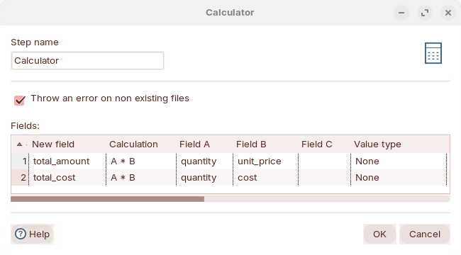
<figure><img src="/files/AGHLdqvc6qoKA35R516L" alt=""><figcaption><p>Calculator</p></figcaption></figure>

**Calculator**

* **Step type:** Transform > Calculator
* **Purpose:** Compute derived fields
* **Configuration:**
  1. Add a **Calculator** step
  2. Add two calculations:

     | New field      | Calculation | Field A    | Field B      |
     | -------------- | ----------- | ---------- | ------------ |
     | `total_amount` | A \* B      | `quantity` | `unit_price` |
     | `total_cost`   | A \* B      | `quantity` | `cost`       |
  3. To compute profit margin, add a **User Defined Java Expression** step (or a second Calculator step) after this one:
     * `profit_margin` = `(total_amount - total_cost) / total_amount`
       {% endtab %}

{% tab title="5. Formula" %}
{% hint style="info" %}

#### **Formula**

The Formula step can calculate Formula Expressions within a data stream. It can be used to create simple calculations like \[A]+\[B] or more complex business logic with a lot of nested if / then logic.
{% endhint %}

1. Drag & drop Formula step onto the canvas.
2. Double-click on the step, and configure the following properties:

<figure><img src="/files/9dejD4TaivkcgrjYg0GM" alt=""><figcaption><p>Formula - profit margin</p></figcaption></figure>

**Formula**

* **Step type:** Scripting > Formula
* **Purpose:** Calculate profit margin using Pentaho Formula Engine (Libformula)
* **Configuration:**
  1. Add a **Formula** step and connect it from the Calculator step
  2. Click **Add** to create a new formula:

     | Field name      | Formula                                          | Value type |
     | --------------- | ------------------------------------------------ | ---------- |
     | `profit_margin` | `[total_amount] - [total_cost] / [total_amount]` | Number     |
  3. The formula uses field references in square brackets (e.g., `[total_amount]`)
  4. This calculates the profit margin as a decimal (e.g., 0.35 = 35% margin)

{% hint style="info" %}
The Formula step uses Pentaho's Libformula engine which supports Excel-like formulas. For simple arithmetic like this, you could also use a Calculator step or User Defined Java Expression. However, Formula steps are more flexible for complex calculations.
{% endhint %}
{% endtab %}

{% tab title="6. Text file output" %}
{% hint style="info" %}

#### **Text file output**

The Text File Output transform exports data to text file formats, most commonly generating CSV files that can be opened in spreadsheet applications like Excel.

This transform also supports creating fixed-width files by specifying field lengths in the fields configuration tab. You have two options for defining the output structure: use an existing Schema Definition or manually configure the field layout. When working with a Schema Definition, pair this transform with the Schema Mapping transform to align your incoming data stream with the chosen schema structure.
{% endhint %}

1. Drag & drop Text file output step onto the canvas.
2. Double-click on the step, and configure the following properties:

<figure><img src="/files/kCugISBUUKErwcVY9zzf" alt=""><figcaption><p>Text file output</p></figcaption></figure>

**Text File Output**

* **Step type:** Output > Text file output
* **Purpose:** Write the processed data to the pdi-output folder
* **Configuration:**
  1. Add a **Text file output** step
  2. Configure the File tab:
     * **Filename:** `~/Jupyter-Notebook/pdi-output/sales_detailed`
     * **Extension:** `csv`
     * **Include date in filename:** Yes
     * **Date time format:** `yyyyMMdd_HHmmss` (produces `sales_detailed_20250218_143022.csv`)
  3. Configure the Content tab:
     * **Separator:** `,`
     * **Header:** Yes
  4. Click **Get Fields** to populate the output field list
     {% endtab %}
     {% endtabs %}
     {% endtab %}

{% tab title="3. File watcher" %}
{% hint style="info" %}

#### File watcher

The file watcher monitors the `pdi-output/` directory and **automatically executes** the analysis notebook inside the Docker container when PDI writes a new file.
{% endhint %}

1. Start File watcher - in a new terminal.

```bash
# Navigate to the scripts directory
cd
cd ~/Jupyter-Notebook/scripts/

# Create a Python virtual environment and install watchdog
# (Modern Linux distros block system-wide pip installs - PEP 668)
python3 -m venv .venv
.venv/bin/pip install watchdog

# Start the file watcher using the venv Python
.venv/bin/python3 file_watcher.py
```

**Expected output:**

```
Watching folder: /home/<user>/Jupyter-Notebook/pdi-output
Press Ctrl+C to stop...
```

2. Re-run the transformation. The file watcher detects the new `sales_detailed.csv` and **auto-executes** the notebook:

<figure><img src="/files/wu3SeUmKy5JHObTInKSc" alt=""><figcaption><p>File watcher</p></figcaption></figure>

{% hint style="info" %}
The file watcher uses `docker exec` to run `jupyter nbconvert --execute` inside the container, so the notebook runs automatically without you having to open Jupyter Lab.
{% endhint %}
{% endtab %}
{% endtabs %}
{% endtab %}

{% tab title="Windows" %}
x

x

x

x

{% tabs %}
{% tab title="1. Jupyter Notebook" %}
{% hint style="info" %}
**Quick Setup**

To check the various scripts and that volume mappings are working, let's analyze a sample sales\_data.csv:

* Install some python packages
* Load a sample dataset - test\_sales\_data.csv
* Run the sales\_analysis.ipynb - check container paths
* Check ouput
  {% endhint %}

{% hint style="danger" %}
Please ensure you have completed the following setup: [Jupyter Notebook](/pentaho-data-integration/setup/data-sources/jupyter-notebook.md).

Check Jupyter Notebook is running in a Docker container ..!
{% endhint %}

{% hint style="info" %}
To list / install python packages:

```docker
cd \
docker exec -it jupyter-datascience bin/bash
```

Once inside the container:

```
pip list - will list the installed packages
```

{% endhint %}

***

1. Install required Python packages:

```
cd \
docker exec -it jupyter-datascience bash
pip install jupyter watchdog xlsxwriter
```

2. Check for the test\_sales\_data.csv & sales\_analysis.ipynb (still in container):

```bash
cd
cd /home/jovyan/datasets
ls
```

```bash
cd
cd /home/jovyan/notebooks
ls
```

3. Open the sales\_analysis.ipynb notebook and RUN each section:

<figure><img src="/files/DbwjvCEhU755peQWs14x" alt=""><figcaption><p>RUN the Notebook</p></figcaption></figure>

4. Check for reports: C:\Jupyter-Notebook\reports\sales\_analysis\_timestamp.xlsx

<figure><img src="/files/4uoibygQV5u5MbqJrB4G" alt=""><figcaption><p>Reports</p></figcaption></figure>

{% hint style="warning" %}
Check you have 2 sheets: Summary & Detailed Data.
{% endhint %}
{% endtab %}

{% tab title="2. File Watcher" %}
{% hint style="info" %}
**File Watcher**
{% endhint %}

x

x

x
{% endtab %}

{% tab title="3. Pentaho Data Integration" %}
{% hint style="info" %}
**Data Pipeline**

The data scientists have deployed the sales\_analysis.ipynb notebook. The notebook will be triggered by a File Watcher that's polling the C:\Jupyter-Notebook\pdi-output for:

* sales\_detailed\_\*.csv

So in this part of the workshop, we're going to create a simple pipeline that:

* Loads the sales.csv
* Cleans and performs some calculations and aggregations
* Outputs to: C:\Jupyter-Notebook\pdi-output folder.
  {% endhint %}

1. Start Pentaho Data Integration.

{% hint style="info" %}
**Windows - PowerShell**

```powershell
Set-Location C:\Pentaho\design-tools\data-integration
.\spoon.bat
```

{% endhint %}

{% hint style="info" %}
**Linux**

```bash
cd
cd ~/Pentaho/design-tools/data-integration
./spoon.sh
```

{% endhint %}

2. Create a New Transformation:

{% tabs %}
{% tab title="CSV File input" %}
{% hint style="info" %}
**CSV File input**

The CSV File Input transform extracts data from delimited files using either a predefined schema or manually configured field layouts. Despite its name, this transform supports any delimiter—pipes, tabs, semicolons, or custom separators—not just commas.

Built for speed through optimized internal processing, this transform offers a focused subset of Text File Input capabilities with three key performance advantages:

**Native I/O (NIO)** uses direct system calls for faster file reading, though it's currently limited to local files without VFS support.

**Parallel Processing** enables distributed file reading when running multiple transform copies or in clustered mode. Each copy processes a separate file block, allowing workload distribution across multiple threads or slave nodes.

**Lazy Conversion** optimizes performance for pass-through data scenarios. When fields flow unchanged from input to output (like file-to-database transfers), this feature prevents unnecessary data type conversions, avoiding the overhead of converting raw data into strings, dates, or numbers.

While this transform has fewer configuration options than the general Text File Input transform, these performance optimizations make it ideal for high-throughput data processing workflows.
{% endhint %}

1. Drag & drop a CSV File input step onto the canvas.
2. Double-click on the step, and configure the following properties:

x

x
{% endtab %}

{% tab title="Data Validator" %}
{% hint style="info" %}
**Data Validator**

The Data Validator transform enables you to define validation rules that check input data across different fields in each row. When the validator encounters a row that violates one or more validation rules, it generates an error or exception.

You can capture all validation errors by configuring an error handling hop from this transform, which will provide you with a comprehensive list of any validation failures that occur during processing.
{% endhint %}

x

x

x
{% endtab %}

{% tab title="Replace in String" %}
{% hint style="info" %}
**Replace in String**

The Replace In String transform performs simple search and replace operations on String fields.

It also supports regular expressions and group references. group references are picked up in the replace by string as $n where n is the number of the group.

You can also use hexadecimal replacements for special characters.
{% endhint %}

x

x

x
{% endtab %}

{% tab title="Calculator" %}
{% hint style="info" %}
**Calculator**

The Calculator transform offers built-in functions that operate on your input field values.

Beyond the function arguments (Field A, Field B, and Field C), you need to define the return type for each function.

After calculations are complete, you can exclude specific fields from the output using the Remove option. This feature helps eliminate temporary values that aren't needed in your final pipeline.

The Calculator delivers significantly faster execution compared to custom JavaScript scripts.
{% endhint %}

x

x

x

x
{% endtab %}

{% tab title="Group By" %}
{% hint style="info" %}
**Group by**

The Group By transform organizes rows from a data source according to one or more specified fields, creating a single row for each distinct group. Additionally, it can compute aggregate values like sums, averages, or counts for each group.

Typical applications include determining average sales figures by product category or tallying inventory quantities for each item type.

This step requires sorted input data to function properly. When working with unsorted data, only identical consecutive rows will be grouped together correctly. Furthermore, if data is sorted externally before entering the Transformation, differences in case sensitivity within the grouping fields may lead to unexpected results.

For scenarios involving unsorted input data, consider using the Memory Group By transform instead, which can handle data regardless of its initial order.
{% endhint %}

x

x

x
{% endtab %}

{% tab title="Text file output" %}
{% hint style="info" %}
**Text file output**

The Text File Output transform exports data to text file formats, most commonly generating CSV files that can be opened in spreadsheet applications like Excel.

This transform also supports creating fixed-width files by specifying field lengths in the fields configuration tab. You have two options for defining the output structure: use an existing Schema Definition or manually configure the field layout. When working with a Schema Definition, pair this transform with the Schema Mapping transform to align your incoming data stream with the chosen schema structure.
{% endhint %}

x

x

x
{% endtab %}
{% endtabs %}

x
{% endtab %}
{% endtabs %}
{% endtab %}
{% endtabs %}


---

# Agent Instructions: Querying This Documentation

If you need additional information that is not directly available in this page, you can query the documentation dynamically by asking a question.

Perform an HTTP GET request on the current page URL with the `ask` query parameter:

```
GET https://academy.pentaho.com/pentaho-data-integration/data-integration/data-sources/jupyter-notebook/pdi-to-jupyter-notebook.md?ask=<question>
```

The question should be specific, self-contained, and written in natural language.
The response will contain a direct answer to the question and relevant excerpts and sources from the documentation.

Use this mechanism when the answer is not explicitly present in the current page, you need clarification or additional context, or you want to retrieve related documentation sections.