# Sales Analysis

{% hint style="warning" %}

#### Workshop - Sales Analysis

The true power of business analytics lies not in creating static reports, but in building dynamic analyses that allow users to explore data from multiple angles, drill into details, and uncover insights on demand. In this comprehensive workshop, you'll master Pentaho Analyzer, the powerful OLAP analysis tool that enables interactive data exploration through drag-and-drop simplicity. You'll learn to create sophisticated pivot table analyses that business users can manipulate in real-time to answer their own questions without returning to IT for new reports.

In this hands-on workshop, you'll experience the full spectrum of Analyzer capabilities, from basic data selection through advanced features like calculated measures, conditional formatting, and drill-through functionality. You'll work with the Steel Wheels sample data to build analyses that reveal sales patterns across territories, product lines, and time periods. You'll learn to enhance your analyses with visual indicators like color scales and data bars, create custom calculations that extend your data model, and implement drill-through links that let users navigate from summary to detail seamlessly. You'll also explore the various visualization options that transform tabular data into compelling charts and graphs, and master the export capabilities that distribute insights across your organization.

**What You'll Accomplish:**

* Understand the three fundamental field types in Analyzer (measures, dimensions, and properties) and how they work together
* Build a pivot table analysis by dragging dimensions to rows and columns and measures to the data area
* Apply multiple filters to restrict analysis to specific territories, time periods, and top performers
* Implement sorting and hierarchical drilling to navigate from years to quarters to months to details
* Add subtotals at multiple levels and grand totals for comprehensive summarization
* Create conditional formatting using color scales, data bars, and trend arrows to highlight patterns
* Build user-defined measures including percentage calculations and custom formulas (Sales plus Tax)
* Enable drill-through links that allow users to view supporting transaction details from summary cells
* Customize column headers, numeric formats, and presentation elements for professional output
* Switch seamlessly between table and chart views (column charts, pie charts, heat grids)
* Export analyses to multiple formats (PDF, Excel, CSV) for distribution and further analysis
* Explore administrative options including XML configuration, MDX query logging, and cache management

By the end of this workshop, you'll have mastered the essential techniques for creating interactive, self-service analyses in Pentaho Analyzer. You'll understand how to structure data dimensionally, how to create calculations that extend your analytical capabilities, and how to format analyses for both visual impact and usability.&#x20;

**Prerequisites:** Pentaho Business Analytics Server with Steel Wheels sample data and configured OLAP schema\
**Estimated Time:** 30 minutes
{% endhint %}

<figure><img src="/files/N4UpVGMjaZWHhHT8tAcK" alt=""><figcaption><p>Analyzer Reports</p></figcaption></figure>

***

{% tabs %}
{% tab title="Leading Product Lines" %}
{% hint style="info" %}

#### Leading Product Lines

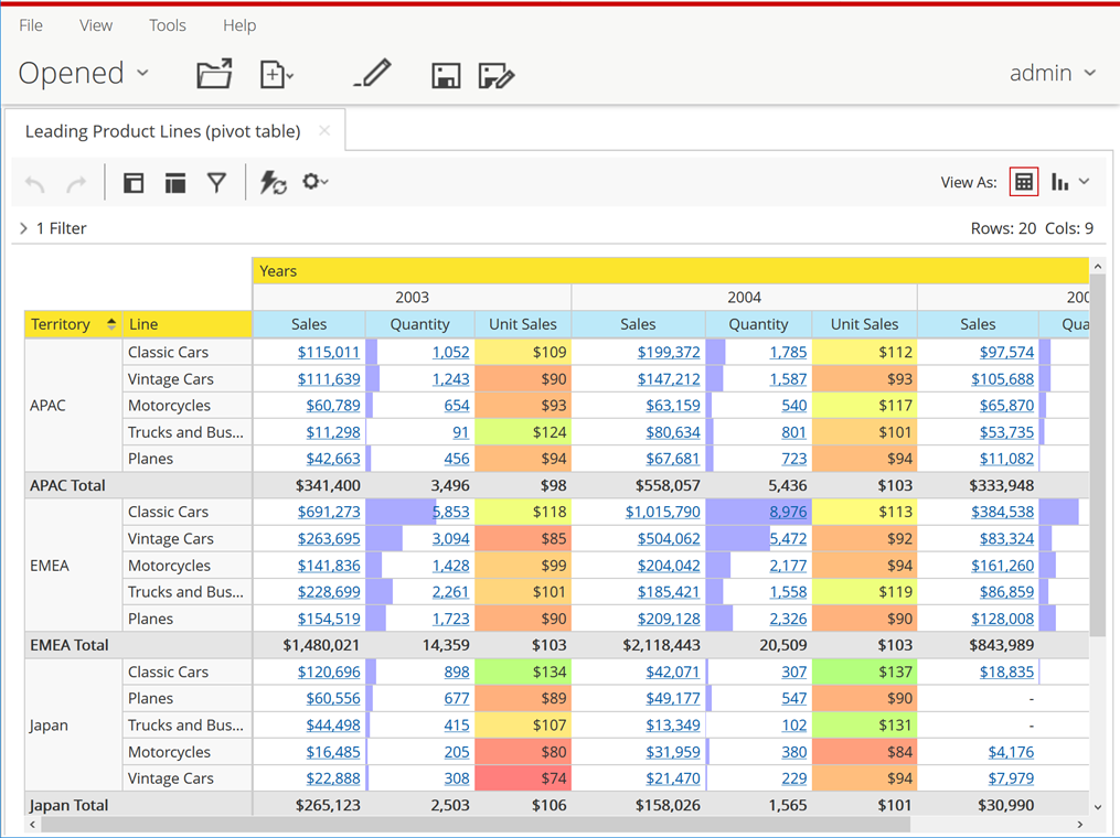
The analysis shows the Sales, Quantity, and Unit Sales for each year by Territory and Line, and includes subtotal lines for each Territory, as well as a grand total line. The Quantity column includes data bars to quickly visualize and compare values.&#x20;

The background colour for the Unit Sales column is formatted using a colour scale range. The report values include hyperlinks allowing you to drill down to the supporting data for each value.
{% endhint %}

1. To open the Leading Product Lines Report, in the Folders pane, expand Public > Steel Wheels, and then in the Files pane, double-click Leading Product Lines (pivot table).

<figure><img src="/files/VcnbCRS3SaYLGynFkaML" alt=""><figcaption><p>Leading Product Lines</p></figcaption></figure>

{% hint style="info" %}
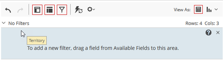
The Interactive Toolbar includes toggle buttons to add more fields to the report, rearrange fields on the report, and show the filters in use. There are also buttons to undo or redo changes.

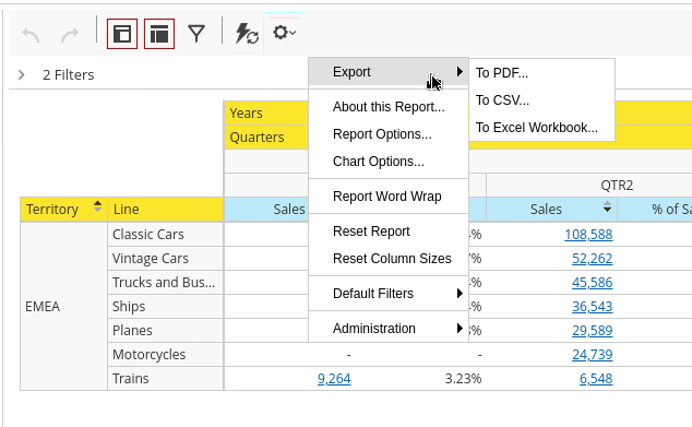
The More actions and options button provides export options, additional report and chart options, and reset options.
{% endhint %}

3. To view the available fields, on the interactive toolbar, click the Add more fields onto the report button.

<div align="center"><figure><img src="/files/rEyQLTnR6eT2AGAaYxib" alt="" width="340"><figcaption><p>Available fields</p></figcaption></figure></div>

{% hint style="info" %}
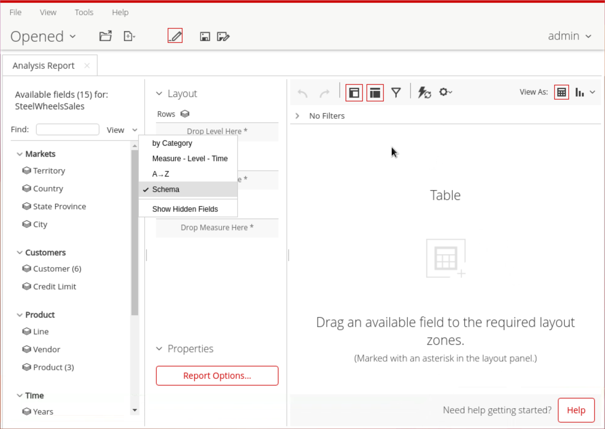
The Available Fields pane shows the data source and the fields available. The fields are listed by category, but you can use the View drop-down list to view the fields by type, alphabetically, or schema.
{% endhint %}

4. To view the Layout panel, on the interactive toolbar, click the Rearrange fields on the report button.

<figure><img src="/files/H7qUFZENcpitcQ96caDU" alt="" width="340"><figcaption><p>Layout</p></figcaption></figure>

{% hint style="info" %}
The Layout panel shows the rows, columns, and measures used in the report. At the bottom is the Report Options button.
{% endhint %}

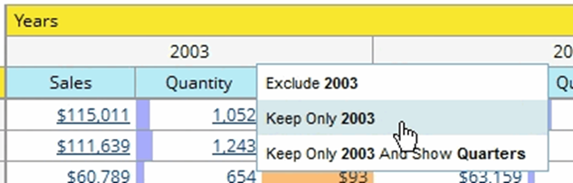
5. To keep only the 2003 data, on the canvas, right-click the 2003 column header, and then click Keep Only 2003.

<figure><img src="/files/Dd89HwwtTCkLGIcNQp9E" alt="" width="475"><figcaption><p>Filter - 2003</p></figcaption></figure>

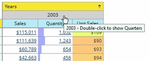
6. To drill down to show the Quarters, on the canvas, double-click the 2003 column header.

<figure><img src="/files/ZeMXx5lCfrIBCH6ANAqQ" alt="" width="450"><figcaption><p>Drill down - Quarters</p></figcaption></figure>

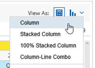
7. To view the analysis as a chart, on the interactive toolbar click the Choose chart type button, and then click Column.

<figure><img src="/files/PKBPiXiIHhyTLK0GP5KX" alt="" width="242"><figcaption><p>Chart options</p></figcaption></figure>

8. To view the report in table format, on the interactive toolbar, click the Switch to table format button.

<figure><img src="/files/Wq22ZgersqlqZvxBxCcl" alt="" width="163"><figcaption><p>Switch to Table format</p></figcaption></figure>

***

{% hint style="info" %}

#### Chart Types

{% endhint %}

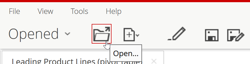
1. To open the Country Performance heat grid, on the main toolbar, click the Open button.

<figure><img src="/files/actq7Jx3UFA1KJmXDNGo" alt="" width="563"><figcaption></figcaption></figure>

2. Navigate to the Public folder, click the Up One Level button twice, and then double-click the Public folder.
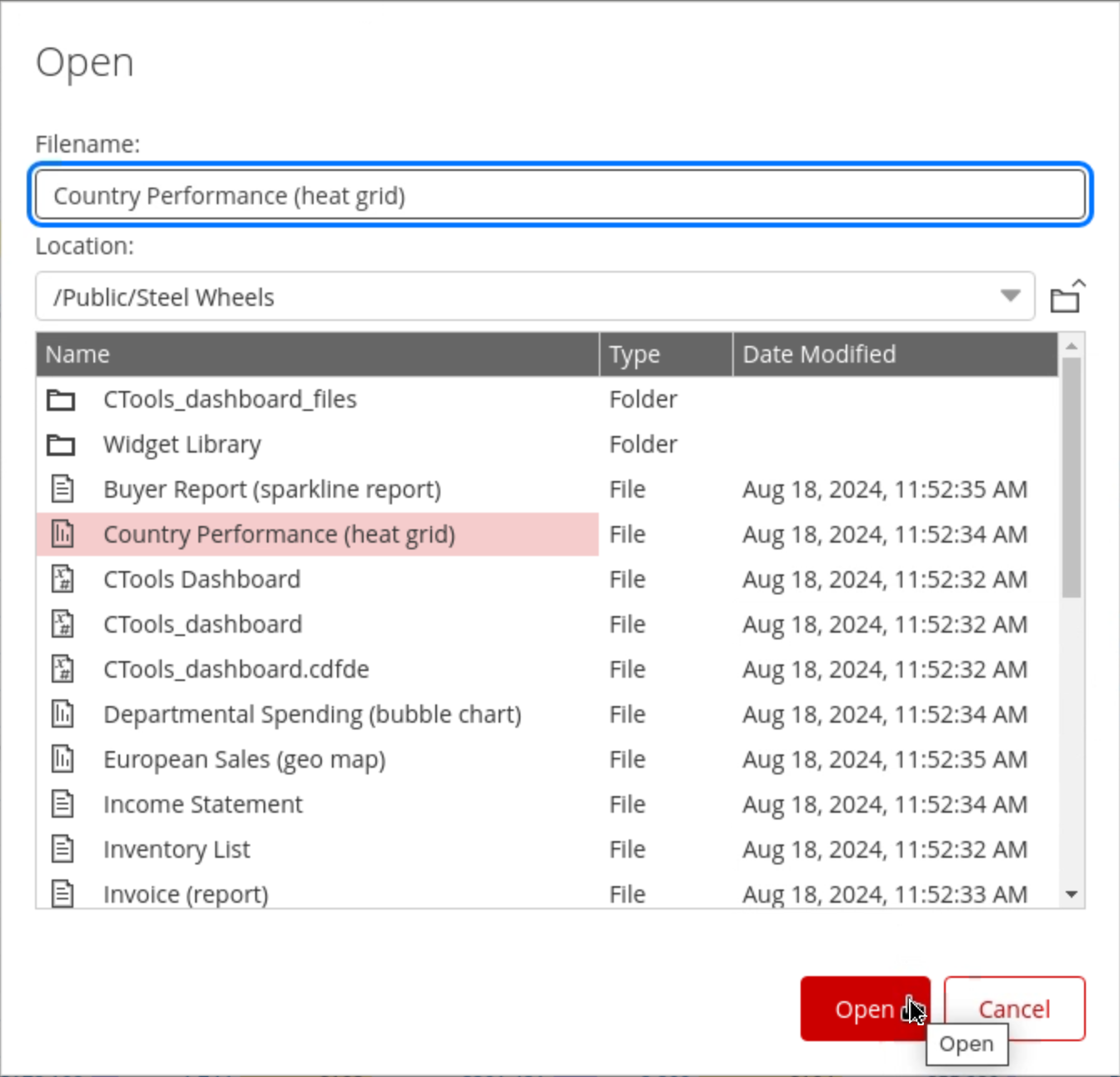
3. Double-click the Steel Wheels folder, then click Country Performance (heat grid), and then click Open.

<figure><img src="/files/h2sXdgVrETcYeGYUMXee" alt=""><figcaption><p>Report List</p></figcaption></figure>

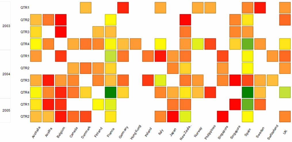
4. View the Country Performance heat grid.

<figure><img src="/files/D6MImZuXnEAnJlTVEXY6" alt=""><figcaption><p>Heat Grid - Country Performance</p></figcaption></figure>

{% hint style="info" %}
The Country Performance heat grid shows Sales by Year and Quarter for each country. The colour coded squares provide a visual representation of the data.

The data for Belgium indicates sales have been consistently low, and sales for France have been fair. We can quickly see that France had a good fourth quarter in 2004, and Spain has had several good quarters.
{% endhint %}

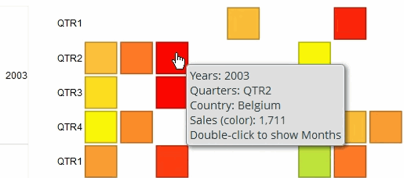
5. To view the underlying details for a specific square, hover the cursor over the red square for Belgium, 2003, QTR2.

<figure><img src="/files/M4GFsQ4gMIyOEqvmSjAw" alt="" width="563"><figcaption><p>Belgium - 2003 - QTR2</p></figcaption></figure>

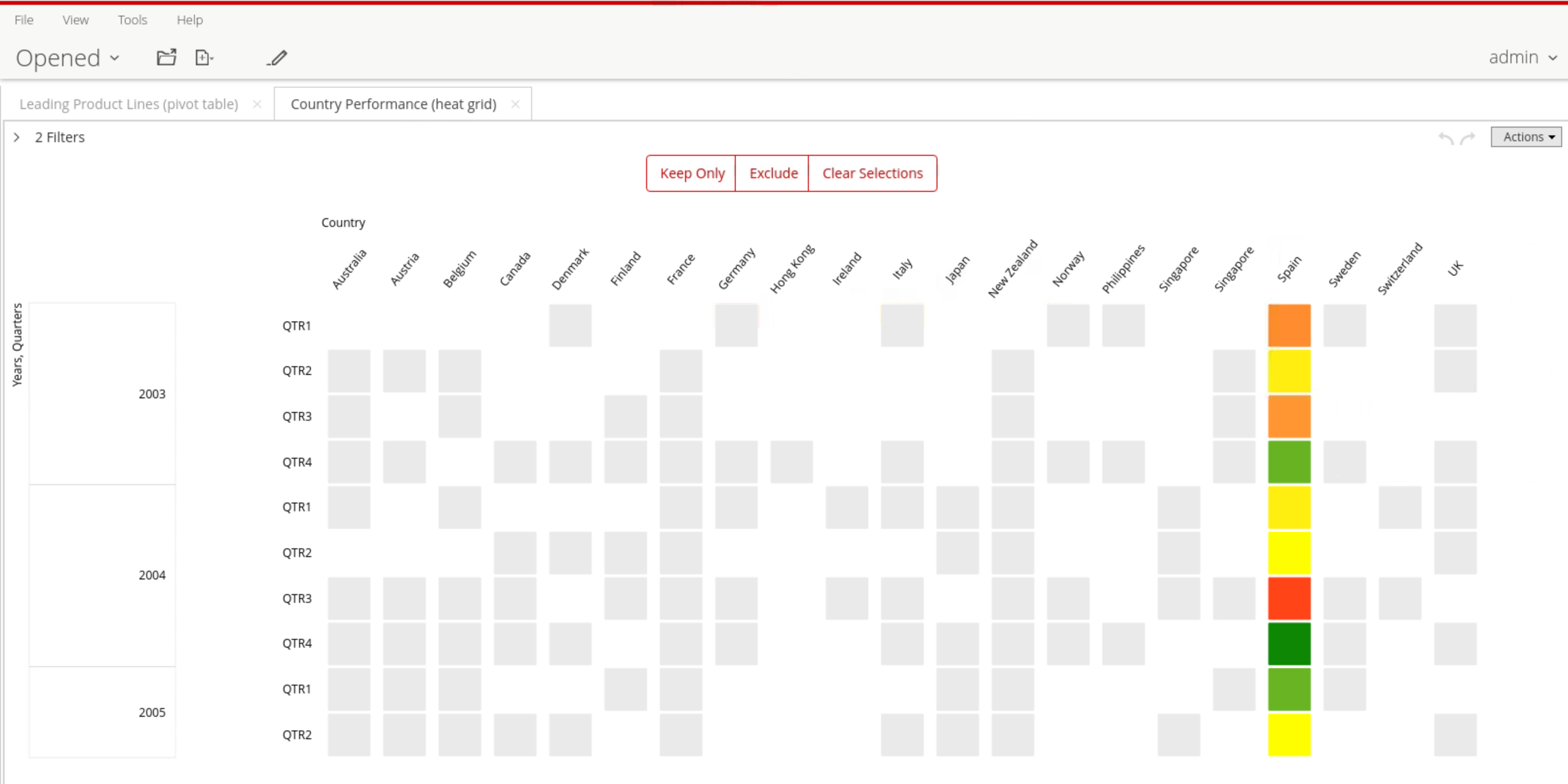
6. Click the Spain label.

<figure><img src="/files/pkAuuSVAzhCRRegfzgrA" alt=""><figcaption><p>Spain data</p></figcaption></figure>

{% hint style="info" %}
The data for Spain is in colour, but the rest of the chart data is dimmed. The buttons to Keep Only, Exclude, and Clear Selections at the top of the heat grid enable you to include / exclude the data selected.
{% endhint %}

7. Drill into the data for Spain at the top of the heat grid, click the Keep Only button.
8. To view the Available Fields and Layout panels, on the interactive toolbar, click the Add more fields onto the report and Rearrange fields on the report buttons.

<figure><img src="/files/AhBTTooNQTaAsrlow8by" alt="" width="332"><figcaption><p>Fields &#x26; Layout</p></figcaption></figure>

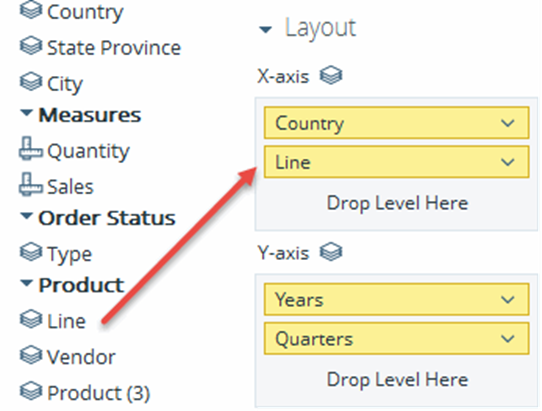
9. To see the sales data for specific product lines in Spain, from the Available Fields pane, select Line and drag it to the X Axis area in the Layout panel.

<figure><img src="/files/ZEg5X8T62xPY063jcgRS" alt="" width="407"><figcaption><p>Add Line</p></figcaption></figure>

{% hint style="info" %}
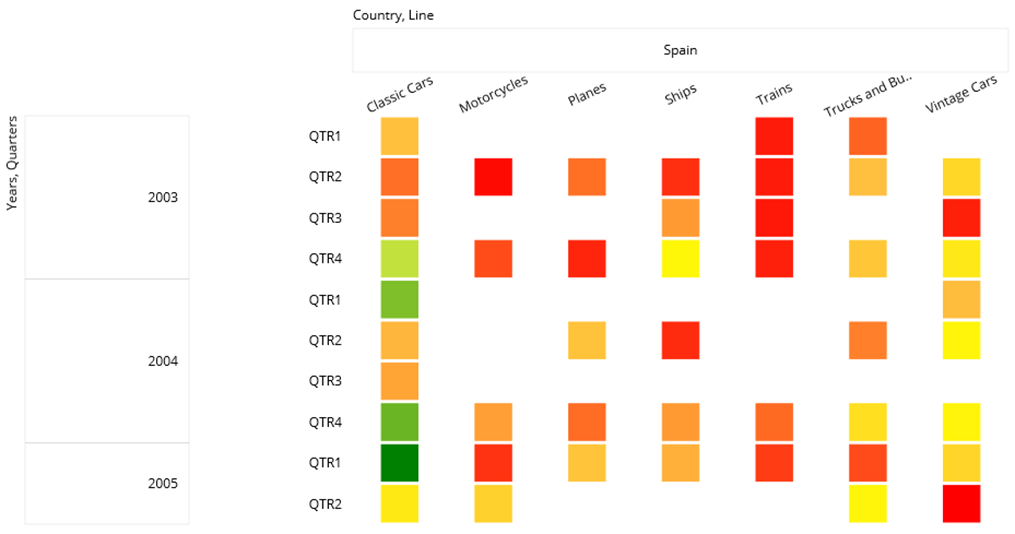
Sales for classic cars were best in Q1 of 2005, but they began to improve in the Q4 of 2004.
{% endhint %}

<figure><img src="/files/YYCjT7vAAjQ7dpx8BfpR" alt=""><figcaption></figcaption></figure>

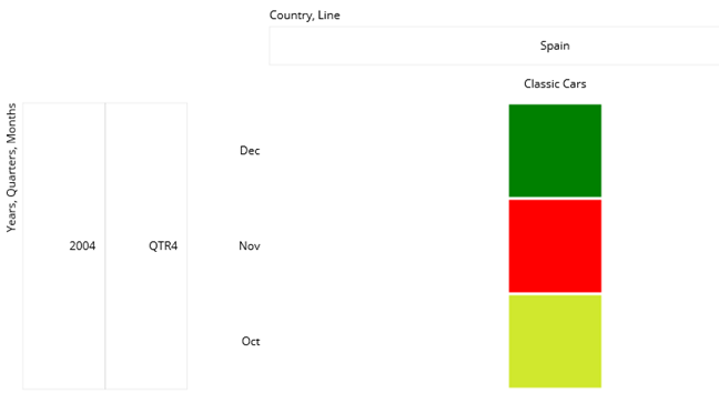
10. Drill down to the months, double-click the green square for Classic Cars, 2004, QTR4. December was the best month of the quarter.

<figure><img src="/files/3lkuwBFOFfgx1nOftv1G" alt=""><figcaption><p>Drill down into Classic Cars, 2004, QTR4</p></figcaption></figure>

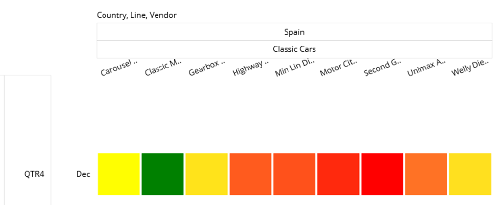
11. Drill down to the Vendor, double-click the green square for December.

<figure><img src="/files/bYognebSq4GCmdsfQ9G1" alt=""><figcaption><p>Drill down into December for Vendor</p></figcaption></figure>

{% hint style="info" %}
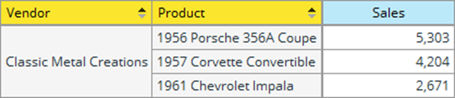
Classic Metal Creations was the highest performing vendor. You could continue drilling down, however, selecting Table will make sense for exporting the sales data.
{% endhint %}

12. On the report title bar, click the View As Table button.

<figure><img src="/files/m7gdpJaEwGA9RWPj9yyb" alt="" width="490"><figcaption><p>Table</p></figcaption></figure>

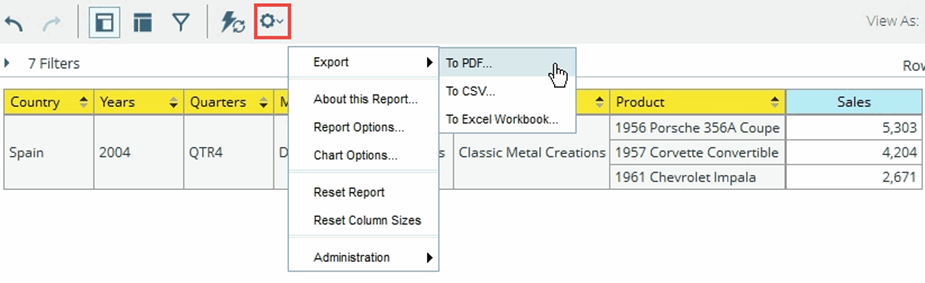
13. On the report toolbar, click More actions and options > Export > To PDF, and then in the Export to PDF window, click Export.

<figure><img src="/files/rOXGw3tSvVslcIjBI82R" alt=""><figcaption><p>Export as PDF</p></figcaption></figure>

{% hint style="info" %}
Selecting PDF opens in a new browser window. You can save or print the PDF using the PDF toolbar.
{% endhint %}

14. Close the PDF browser window.
15. On the report toolbar click More actions and options > Reset.
    {% endtab %}

{% tab title="Sales Analysis" %}
{% hint style="info" %}

#### Sales Analysis

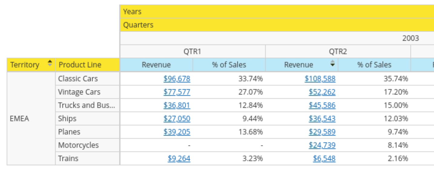
The report will display Sales Revenue grouped by Territory and Product Line over time.
{% endhint %}

<figure><img src="/files/tBGCxEvsy1uPmyLDTkiA" alt=""><figcaption><p>Final Table - EMEA: Revenue by Product Line Yr2003</p></figcaption></figure>

{% tabs %}
{% tab title="Data Source" %}
{% hint style="info" %}

{% endhint %}

1. From the User Console Home Perspective, click Create New > Analysis Report.
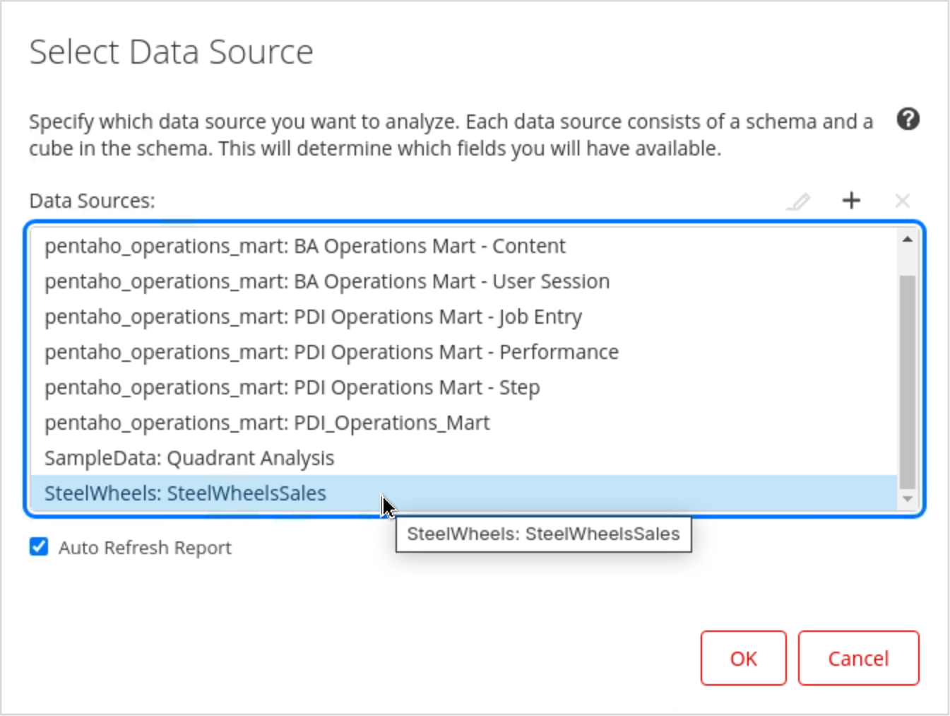
2. In the Select Data Source window, click Steel Wheels: SteelWheelsSales, and then click OK.

<figure><img src="/files/8KQ6XN6ja75zzWY39SHY" alt="" width="563"><figcaption><p>SteelWheels: SteelWheelsSales</p></figcaption></figure>

***

{% hint style="info" %}
**Data Types**

When you first open Analyzer, the available fields associated with the data source you select are displayed in the Available Fields panel.

The Available Fields panel consists of a list of measures and dimensions.

&#x20; • Measures: consist of the numeric data that can be calculated, and are depicted with the ruler icon.

&#x20; • Dimensions: are different aspects of the calculated data, and are depicted with the stacked squares icon. If a dimension has a number in parenthesis next to it, this indicates it has associated properties.

&#x20; • Properties: are single data items related to a database object. The database schema associates one or more properties with each database entity.  For example, the dimension ‘Product’ can have the properties: colour, shape, size, weight, etc..
{% endhint %}

<figure><img src="/files/ieR3va5lOYsRY3erWgtb" alt=""><figcaption></figcaption></figure>

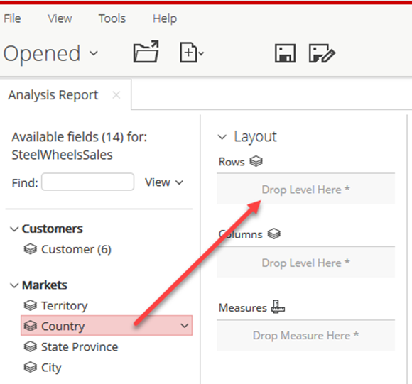
1. From the Available Fields panel, select Country and drag it to the Rows drop zone on the Layout panel.

<figure><img src="/files/tum9tWpzYHTdaD8h814n" alt="" width="435"><figcaption><p>Add Country field</p></figcaption></figure>

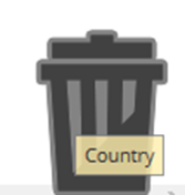
2. To remove Country, from the canvas:

   ·        Click the Country header.

   ·        Drag it to the lower right corner of the canvas.

   ·        Drop it in the trashcan.

<figure><img src="/files/OkjRUuIcfo7qp4P5V8Nd" alt="" width="125"><figcaption></figcaption></figure>

3. Add Sales to the report by dragging it to the Measures drop zone on the Layout panel.
4. From the Available Fields panel, double-click Territory.
5. Select Years and drag it to the Columns drop zone on the Layout panel.
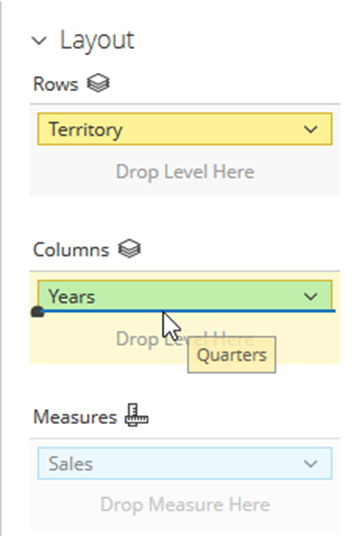
6. Select Quarters and drag it to the Columns drop zone on the Layout panel. Drop Quarters *below* Years.

<figure><img src="/files/TaQVwEbky3d6GVfulvLq" alt="" width="269"><figcaption></figcaption></figure>

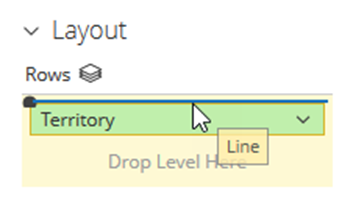
7. Select Line and drag it to the Rows drop zone on the Layout panel. Drop Line *above* Territory.

<figure><img src="/files/w04CVC5OeMS3bJpzhrM8" alt="" width="265"><figcaption></figcaption></figure>

{% hint style="info" %}
When you add columns and rows Analyzer dynamically aggregates the Measure to the required level.
{% endhint %}

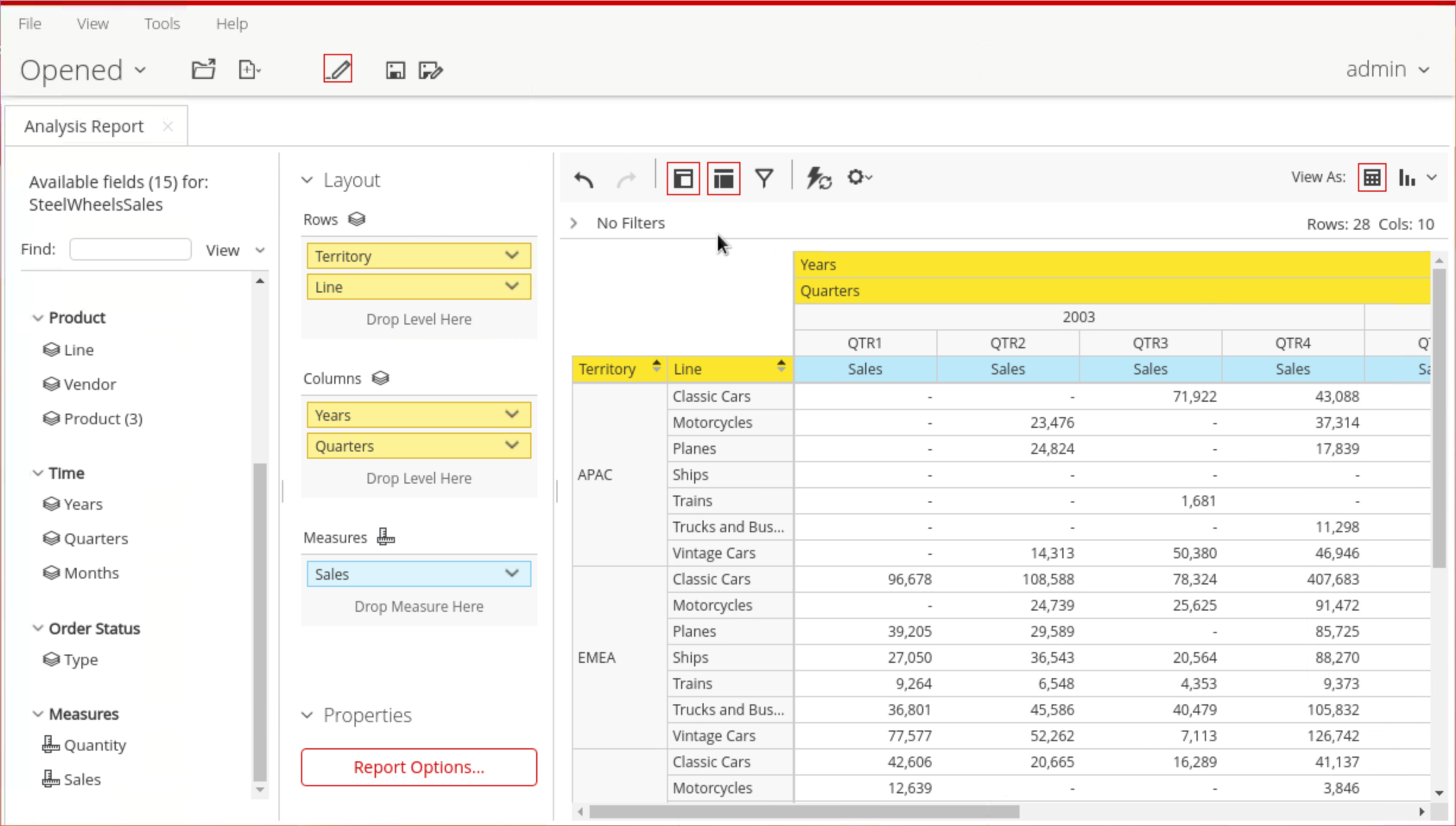
8. To rearrange the fields, on the Layout panel, click Territory and drag it *above* Line.

<figure><img src="/files/m4JrYI9ZI03SeHsYpYHL" alt=""><figcaption><p>Report - Territory Sales Analysis</p></figcaption></figure>
{% endtab %}

{% tab title="Filter & Conditional Formatting" %}
{% hint style="info" %}
Filters are used to restrict or limit the data that is presented in an analysis. When you create a filter for a text field you can select from a list of values or match a specific value by typing the value in the text box and specifying a constraint (Contains or Does not Contain).&#x20;

When you filter on time periods you can choose a commonly used time period, select from a list, or select a range.
{% endhint %}

1. On the Interactive Toolbar, click the Filter button.

<figure><img src="/files/fECpxyE7hw7PZR5gEkos" alt=""><figcaption><p>Filter option</p></figcaption></figure>

2. In the Available Fields panel, select Territory and drag it to the Filter panel.

<figure><img src="/files/o9OLWdtoT597xFuqtSgM" alt=""><figcaption><p>Filter Panel</p></figcaption></figure>

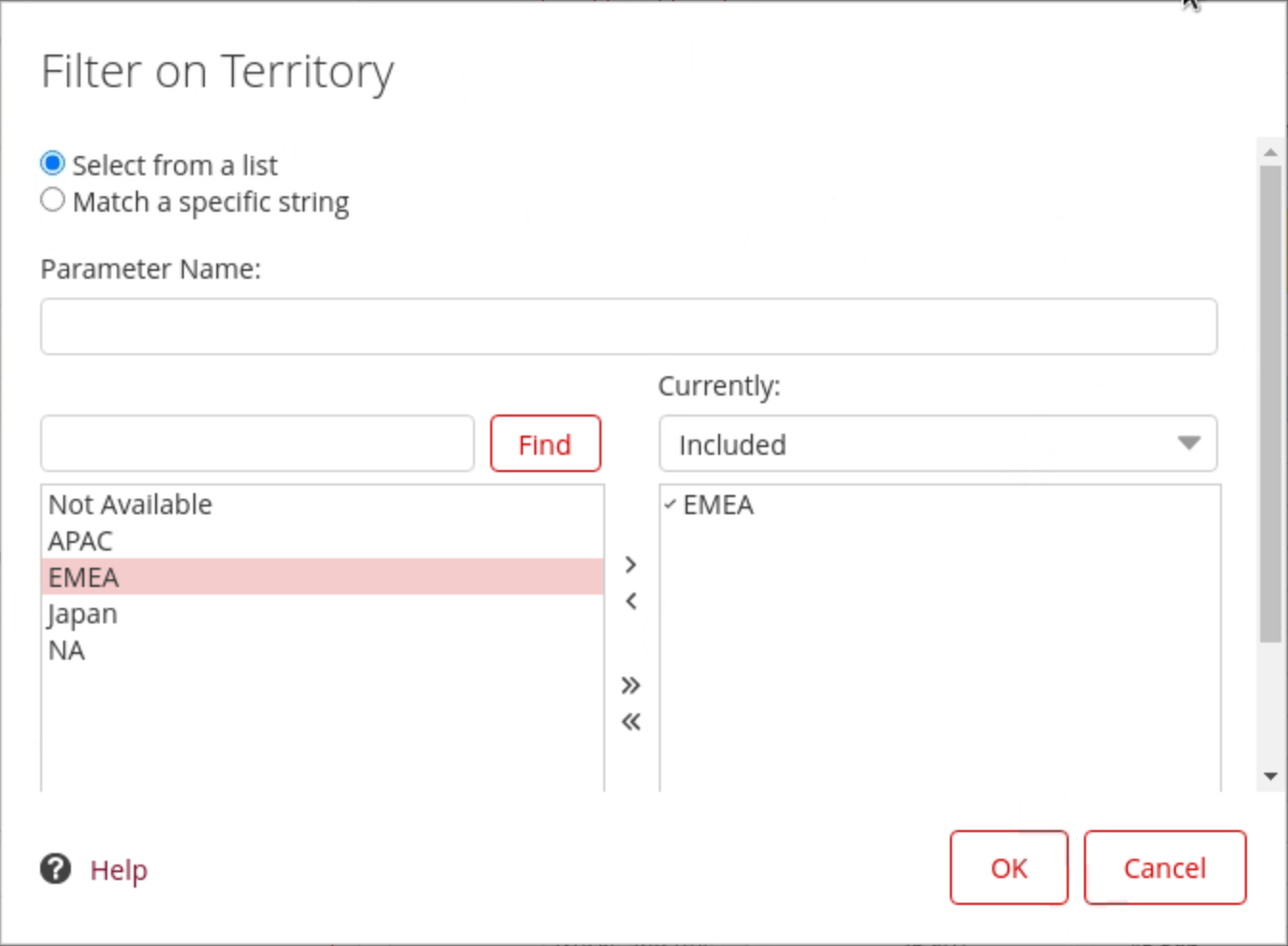
3. To display only EMEA, in the Filter on Territory dialog box:

   &#x20; • Select: Select from a list.

   &#x20; • From the list of values, click EMEA.

   &#x20; • Click the right arrow to move EMEA to the Currently Included list.

   &#x20; • Click OK.

<figure><img src="/files/pkGUJ1vwO5mdhK3o1etI" alt=""><figcaption><p>Filter - EMEA</p></figcaption></figure>

{% hint style="info" %}
The Parameter Name field enables you to define the filter as a prompt.&#x20;
{% endhint %}

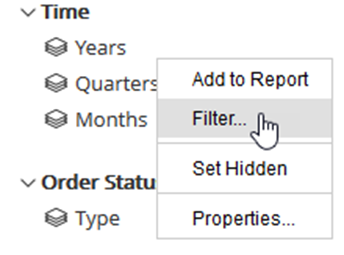
4. In the Available Fields panel, right-click Years, and then select Filter.

<figure><img src="/files/IBBfNvFNXA8Jlrvdv3RA" alt="" width="258"><figcaption><p>Filter - Years</p></figcaption></figure>

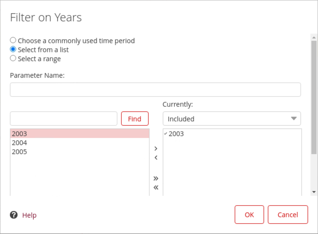
5. To display only 2003, in the Filter on Years dialog box:

   &#x20; • Select: Select from a list.

   &#x20; • From the list of values, click 2003.

   &#x20; • Click the right arrow to move 2003 to the Currently Included list.

   &#x20; • Click OK.

<figure><img src="/files/Jmd2DSsPvGcfMvvMU1yw" alt=""><figcaption><p>Filter - 2003</p></figcaption></figure>

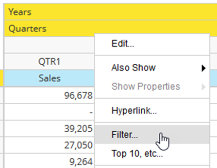
6. In the analysis canvas, right-click Quarters, and then select Filter.

<figure><img src="/files/EnxPQeonKCbkeu3lDQ1f" alt="" width="335"><figcaption><p>Filter - Quarters</p></figcaption></figure>

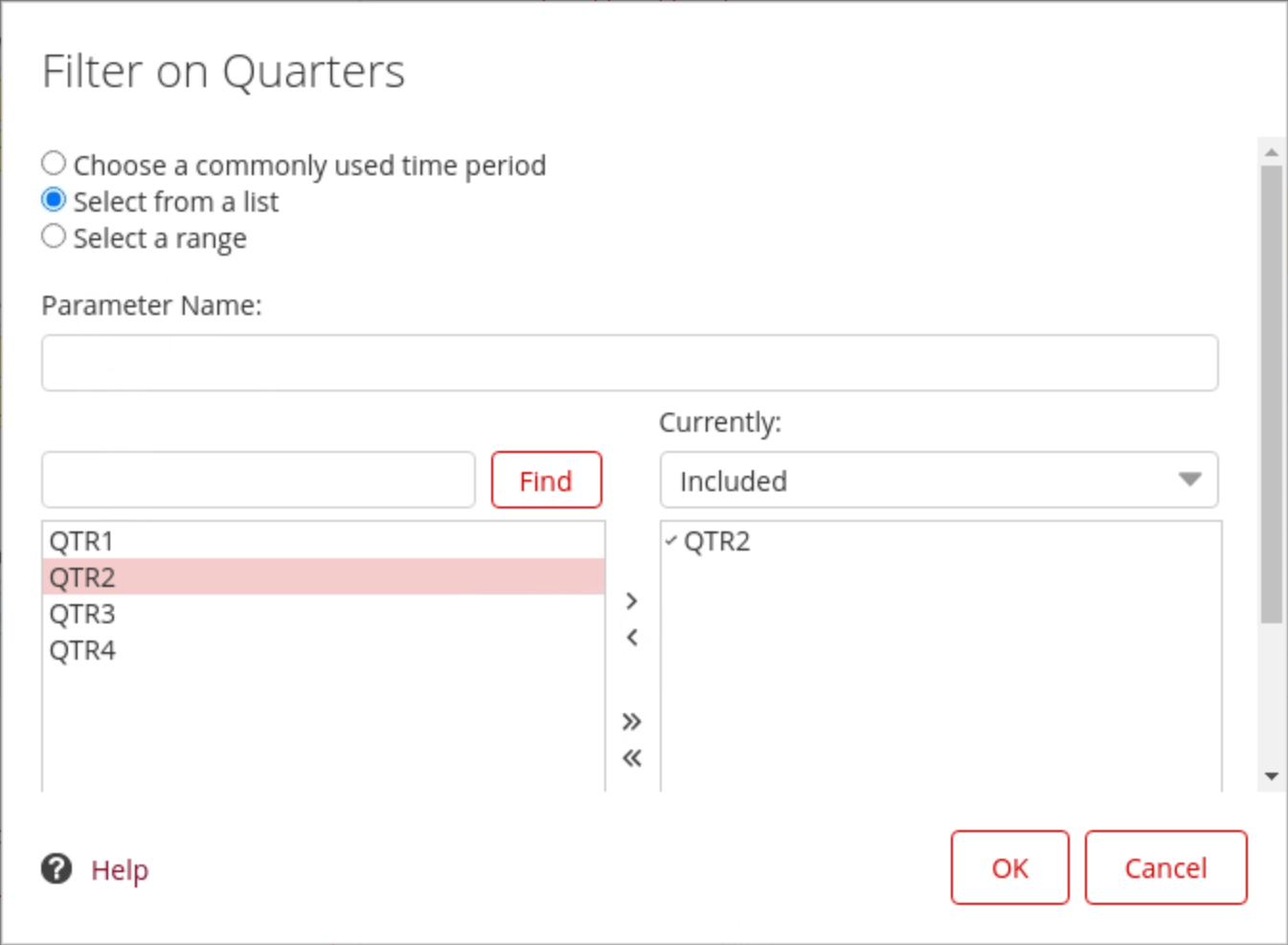
7. To display only the second quarter, in the Filter on Quarters dialog box, select: Select from a list.

<figure><img src="/files/lNxQCSnjhsvc9FuY7MxC" alt=""><figcaption><p>Filter - QTR 2</p></figcaption></figure>

8. From the list of values, click QTR2, then click the right arrow to move QTR2 to the Currently Included list, and then click OK.

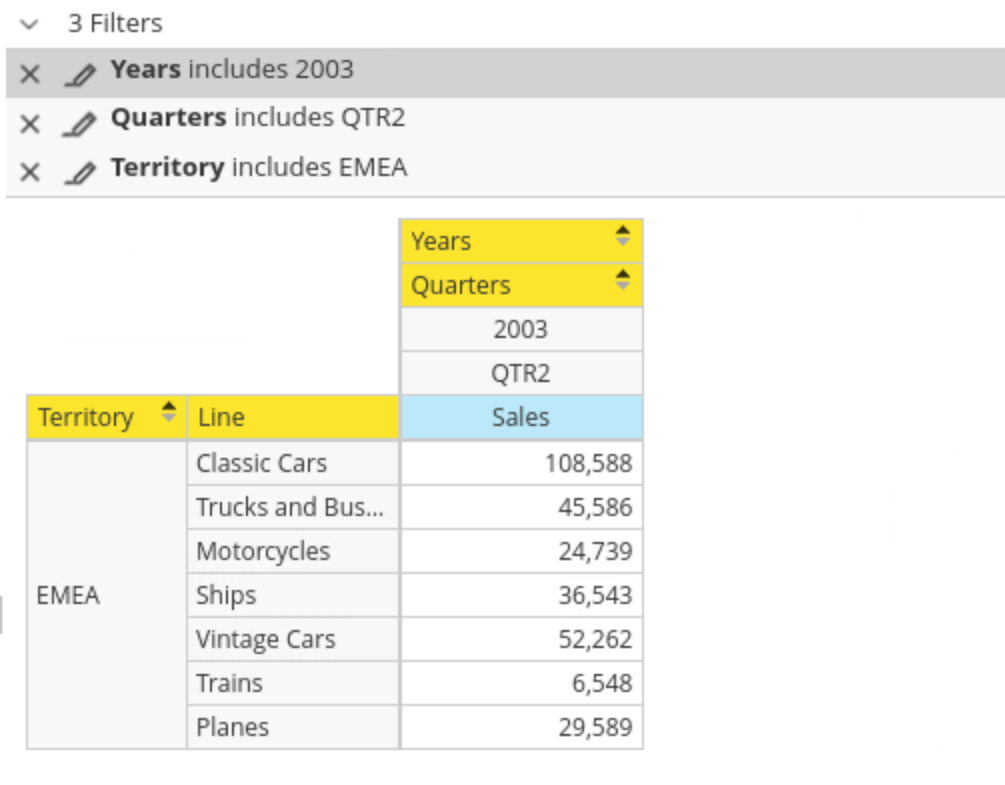
<figure><img src="/files/1WFN4UO4VnO2BFlJneWY" alt="" width="563"><figcaption><p>Filters</p></figcaption></figure>

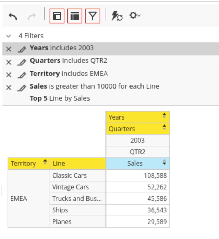
9. On the analysis canvas, click Sales and drag it *up* to the Filter panel.
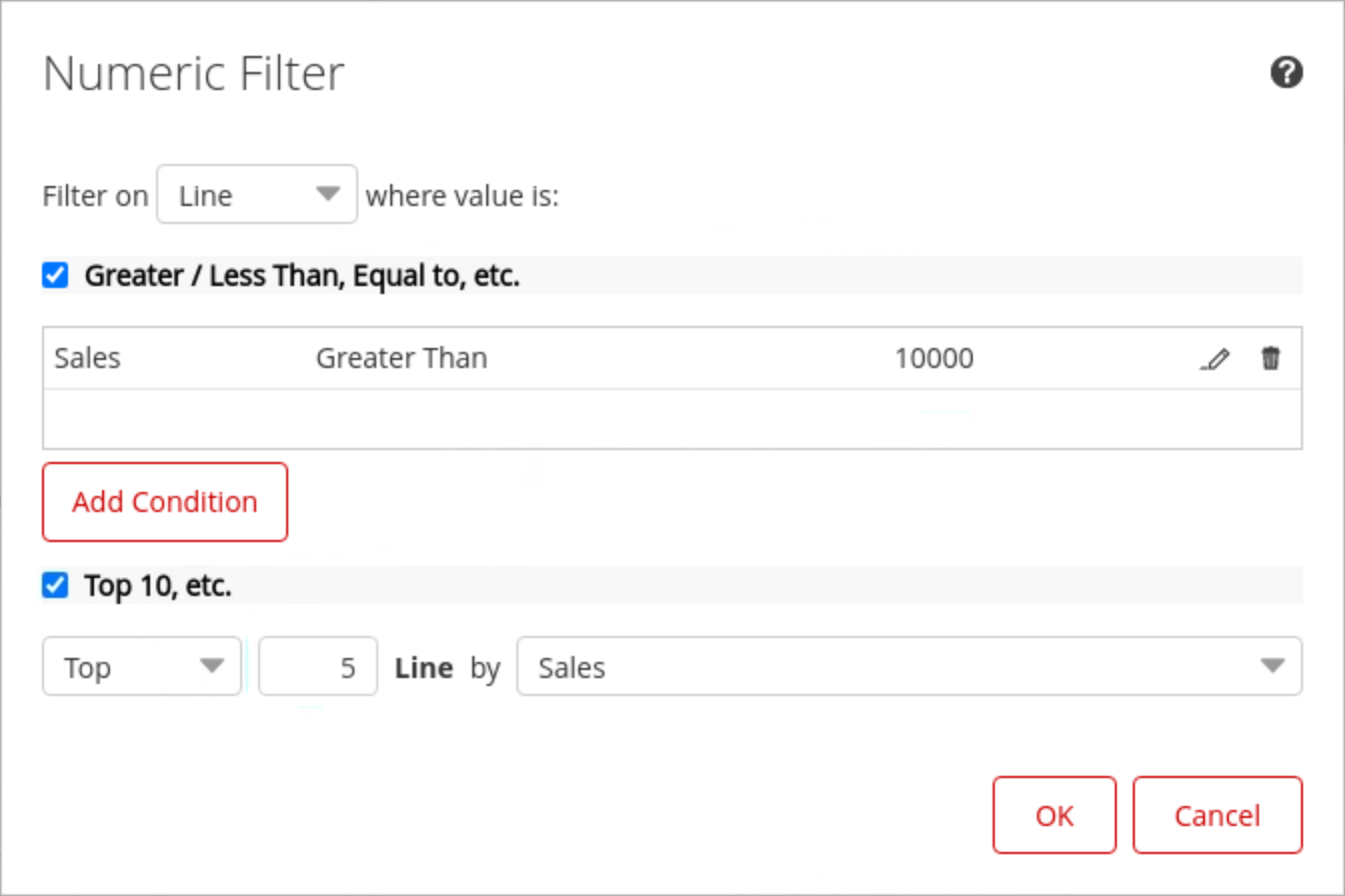
10. To display the Top 5 Product Lines with Sales Greater Than 10,000 in the Filter on Sales dialog box:

    &#x20; • In the text box for Sales Greater Than, type: 10000.

    &#x20; • Click the Top 10, etc. check box..

    &#x20; • In the numeric value box, type 5.

    &#x20; • Click OK.

<figure><img src="/files/Uv5gVV0JBu9q3UOcPvdP" alt=""><figcaption><p>Numeric Filter - Top 5 Lines by Sales</p></figcaption></figure>

<figure><img src="/files/Tua671KH645HwGJPp7Qi" alt="" width="375"><figcaption><p>EMEA: Top 5 Product Lines by Sales 2003 QTR2</p></figcaption></figure>

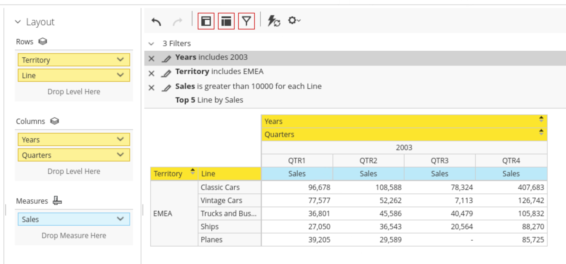
11. On the analysis canvas, right-click the QTR2 header for 2003, and then select Show All Quarters.
12. Remove the Sales is greater than 10000 filter.

<figure><img src="/files/4nHezMN6L12EW06F7ygL" alt=""><figcaption><p>EMEA: Top 5 Product Line by Sales for 2003</p></figcaption></figure>

***

{% hint style="info" %}
**Applying Conditional Formatting**

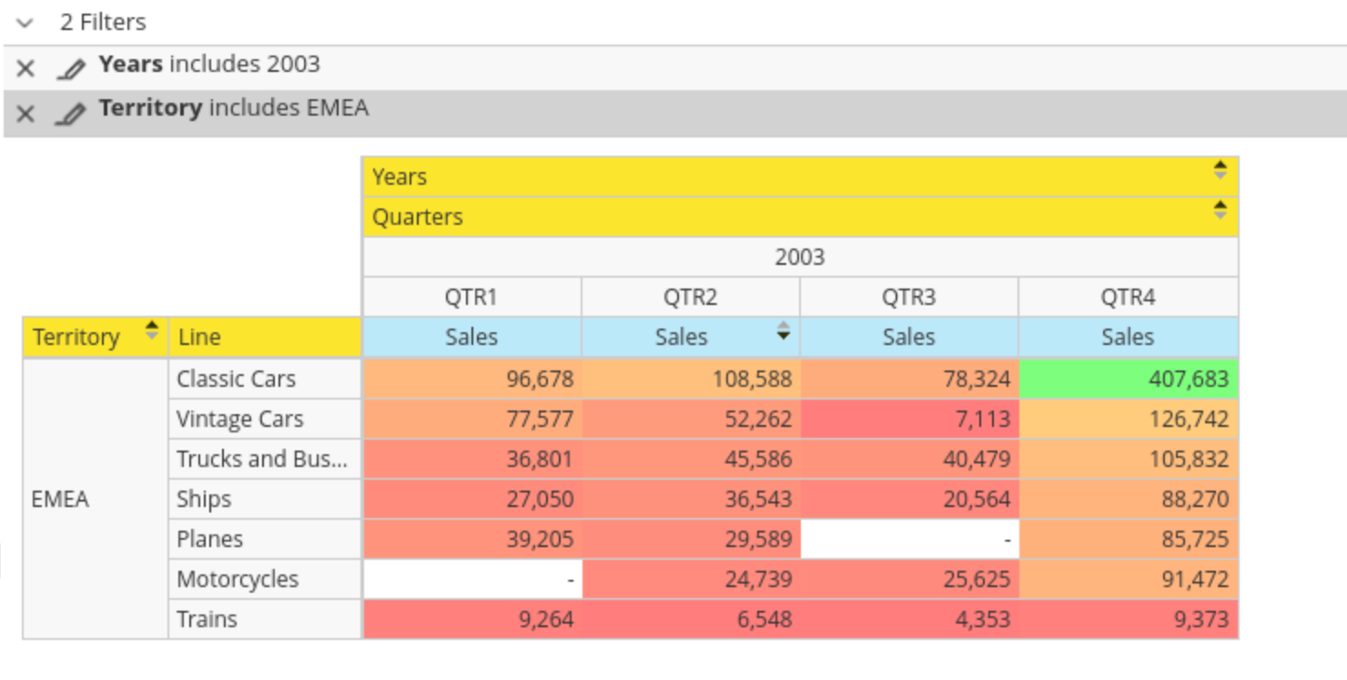
Conditional formatting means that cells within the analysis will be physically affected by the data they contain. The most common form of conditional formatting is stoplight reporting, where cell backgrounds are coloured red, green, or yellow depending on user-defined thresholds.

Analyzer provides the following methods for conditionally formatting numeric data:

&#x20; • Color Scale

&#x20; • Data Bar

&#x20; • Trend Arrow
{% endhint %}

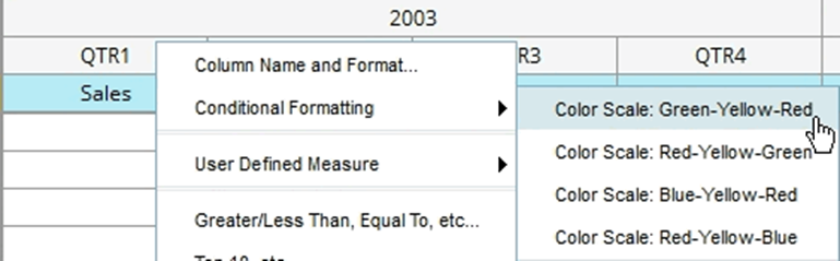
1. Right-click one of the Sales headers, and then select Conditional Formatting > Color Scale: Green-Yellow-Red.

<figure><img src="/files/dIRH9BPKznRvTv1RAj27" alt="" width="563"><figcaption><p>Apply Conditional Formatting</p></figcaption></figure>

<figure><img src="/files/v03RZBeIQgMnf1DDfHC3" alt=""><figcaption><p>Conditional Formatting</p></figcaption></figure>

2. Remove the conditional formatting, right-click one of the Sales headers, and then deselect Conditional Formatting >  Green-Yellow-Red.
   {% endtab %}

{% tab title="Calculations & Drill-Through" %}
{% hint style="info" %}
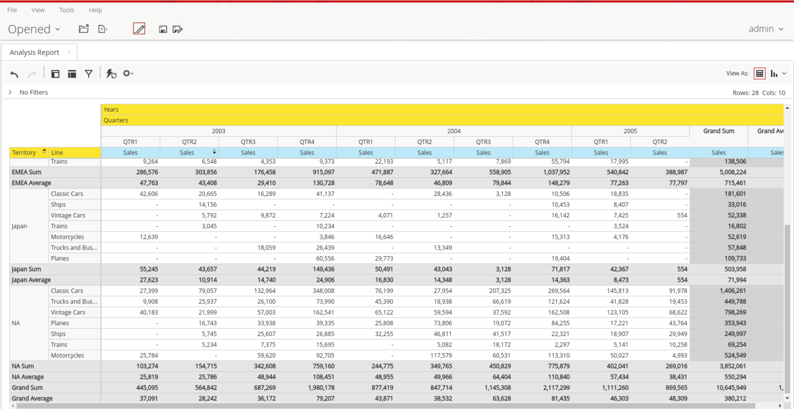
Grand totals and subtotals summarize detail row or column values. You can choose to summarize the data in the following ways:

&#x20; • Aggregate

&#x20; • Sum

&#x20; • Average

&#x20; • Max

&#x20; • Min
{% endhint %}

1. Remove all Filters.
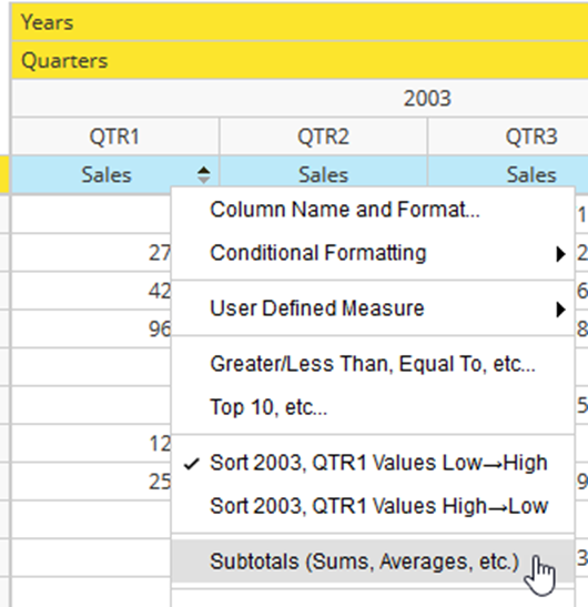
2. In the analysis details, right-click one of the Sales headers, then select Subtotals (Sums, Averages, etc.).

<figure><img src="/files/8RfWLIiKamWToZh085Hn" alt="" width="398"><figcaption><p>Subtotals</p></figcaption></figure>

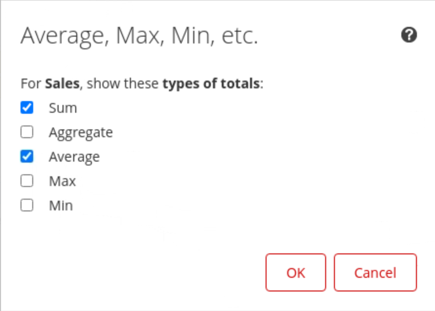
2. Select Average, and then click OK.

<figure><img src="/files/zOIFwzbQNjXBo2F3GP95" alt="" width="375"><figcaption><p>Calculations</p></figcaption></figure>

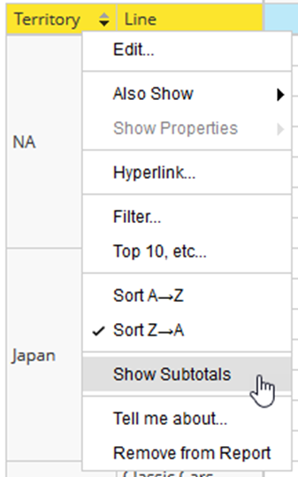
3. In the analysis details, right-click the Territory header, and then select Show Subtotals.

<figure><img src="/files/j8NOdgJAmEPrClg8UM8J" alt="" width="253"><figcaption><p>Show Subtotals</p></figcaption></figure>

{% hint style="info" %}
Subtotals do not appear in the analysis, until the dimension selected.
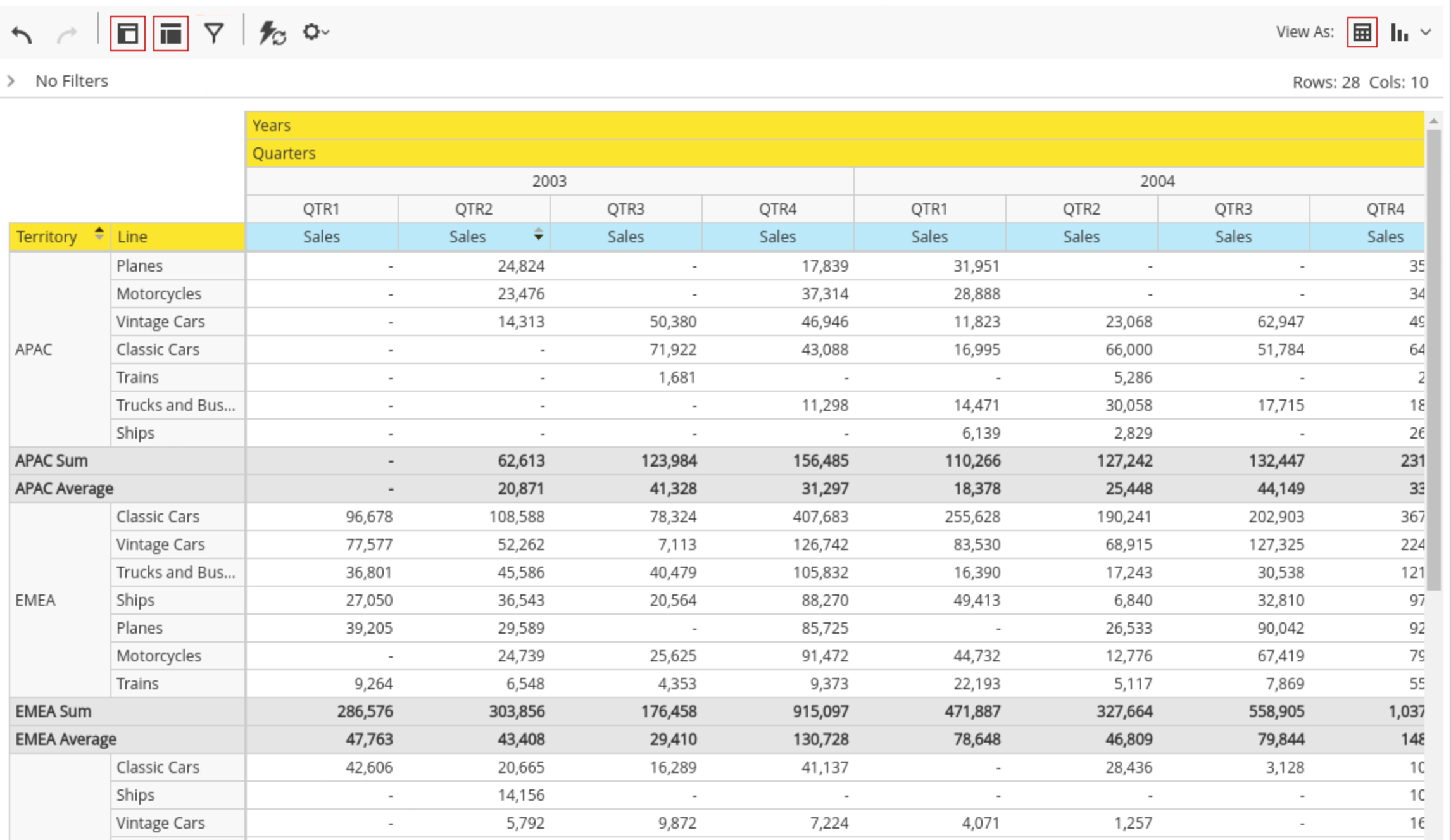
{% endhint %}

<figure><img src="/files/mMXOrPVbtfgKUFtRnaMr" alt=""><figcaption><p>Subtotals &#x26; Averages</p></figcaption></figure>

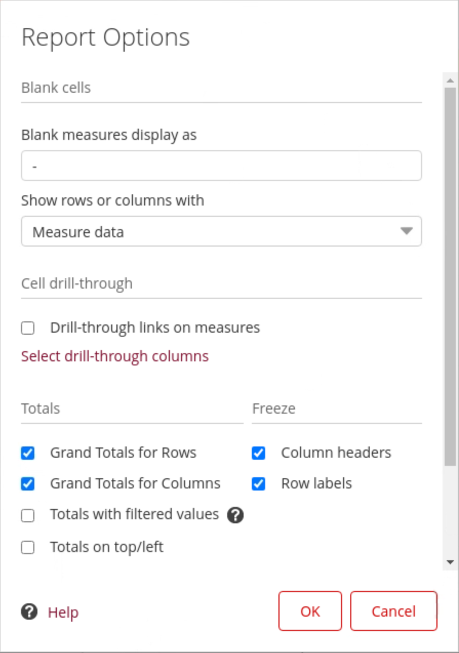
4. To show grand totals for columns and rows, from the Layout panel: Click Report Options.
5. In the Report Options window, select Show Grand Totals for Rows and Show Grand Totals for Columns.

<figure><img src="/files/5IC2cN8x5qMPwGbtWX6i" alt="" width="375"><figcaption><p>Grand Totals - Rows &#x26; Columns</p></figcaption></figure>

4. Click OK.

<figure><img src="/files/CenVRwiKWi2tbMysG8y9" alt=""><figcaption><p>Grand Totals for Rows &#x26; Columns</p></figcaption></figure>

***

#### User Defined Measure

{% hint style="info" %}
Analyzer allows you to create three types of measures directly within an analysis:

&#x20; • Percent of, rank, running sum, or percent of running sum

&#x20; • Calculated Measures

&#x20; • Trend Measures

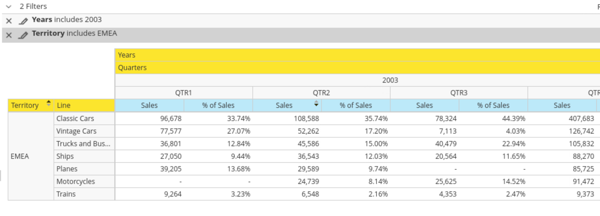
So we're going to display the percent of sales for each product line, and add a simple calculated measure to show the sales plus 6% tax.
{% endhint %}

1. Remove all Totals, Subtotals & Averages for rows & columns.
2. Apply 2 filters:

&#x20;      • Territory: EMEA&#x20;

&#x20;      • Year 2003

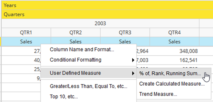
3. Right-click one of the Sales headers, then select User Defined Measure > % of, Rank, Running Sum….

<figure><img src="/files/gpdHY9iq9A1YyGIGWJBO" alt="" width="563"><figcaption><p>User Defined Measure</p></figcaption></figure>

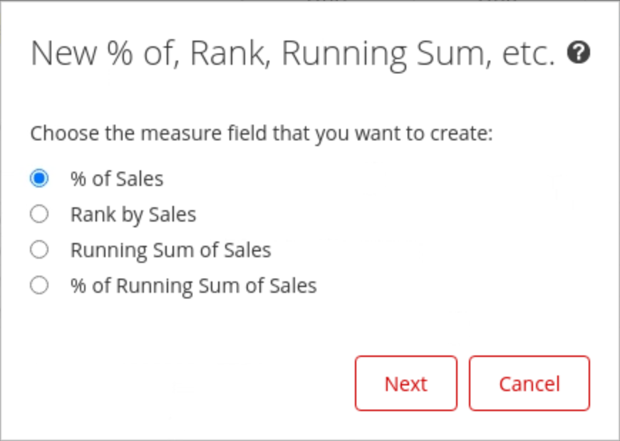
4. Select: % of Sales.

<figure><img src="/files/kmsS9rKUsgcOLEGVC74k" alt="" width="375"><figcaption><p>% of Sales</p></figcaption></figure>

5. Click Next.
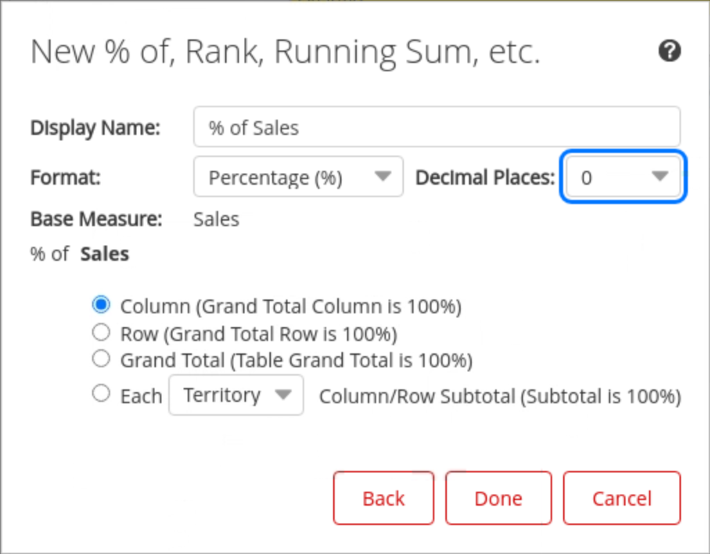
6. Click the drop-down arrow for Decimal Places, select 0.

<figure><img src="/files/hSlUkxg4b6po22IECwhs" alt="" width="375"><figcaption><p>% of Sales</p></figcaption></figure>

7. Click: Done.

<figure><img src="/files/MrXCjiBis7GXYX2Dvgqf" alt=""><figcaption><p>% of Sales</p></figcaption></figure>

***

#### Calculated Measure

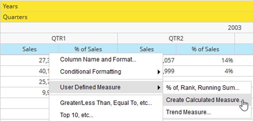
1. In the analysis details right-click one of the Sales headers, then select User Defined Measure > Create Calculated Measure.

<figure><img src="/files/YXTsIvusL8BwgYTTeoMQ" alt="" width="563"><figcaption><p>Calculated Measure</p></figcaption></figure>

{% hint style="info" %}
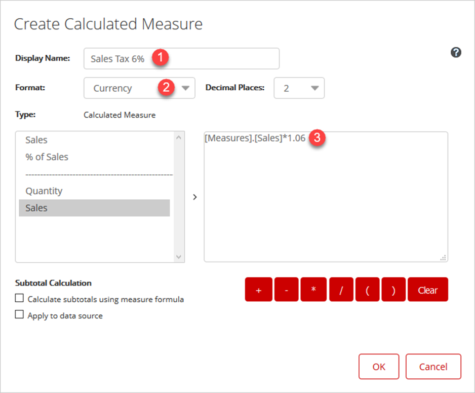
The left panel lists the measure fields available to use in the calculation. The Selection pane is where you write the MDX expression to calculate the new measure.
{% endhint %}

<figure><img src="/files/EhRy9fZbrSNGlJPXkB1q" alt=""><figcaption><p>Calculated Measure - 6% Tax</p></figcaption></figure>

2. In the Name text box, type Sales + 6% Tax.
3. To specify the numeric format:
4. Click the drop-down arrow for Format.

&#x20;      • Select Currency.

&#x20;      • Click the drop-down arrow for Decimal Places.

&#x20;      • Select 0.

5. To multiply Sales by 1.06, in the formula pane:

&#x20;      • Click to the right of sales.

&#x20;      • Type: \* 1.06.

&#x20;      • Click OK.

<figure><img src="/files/TE9eKBtloDRwZM6ooqhN" alt=""><figcaption><p>Sales + 6% Tax</p></figcaption></figure>

***

#### Drill-Through

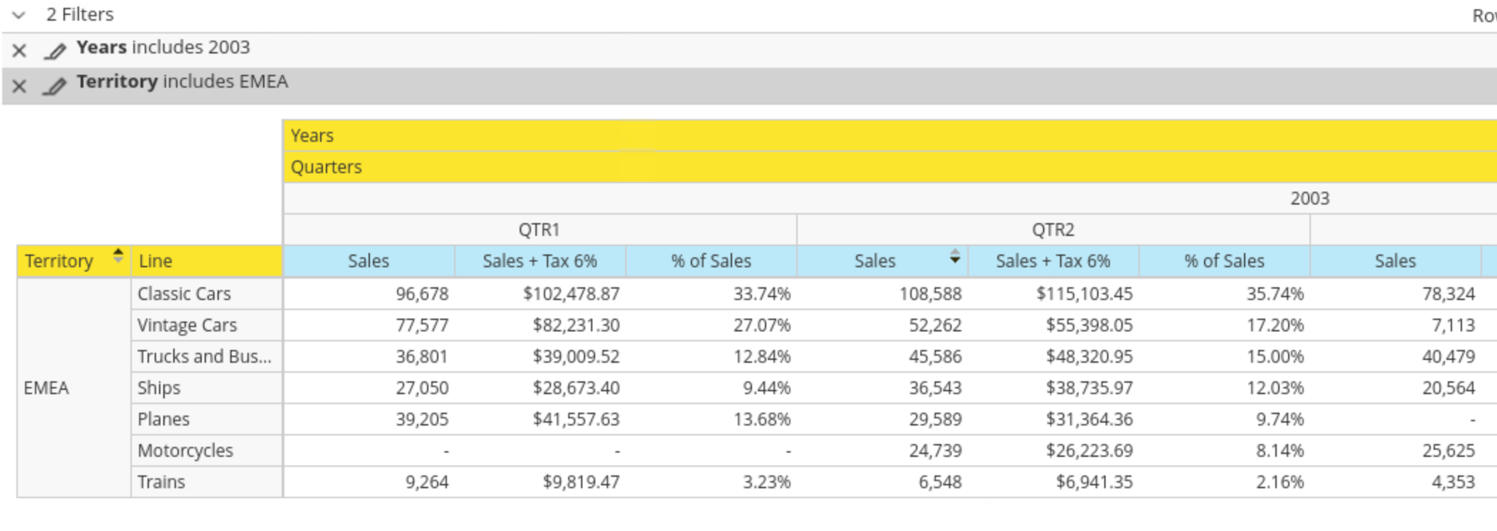
{% hint style="info" %}
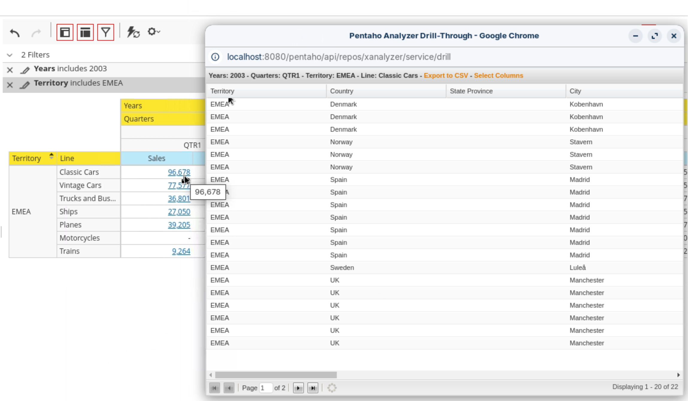
To create reports based on specific measure data, you can implement drill through links in Analyzer. This will turn all non-calculated measures into links which, when clicked, open a data table that enables you to quickly view more details for that data point.
{% endhint %}

1. Remove the following columns:

&#x20;       • Sales + Tax 6%

&#x20;       • % of Sales

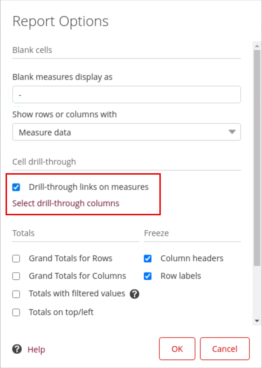
2. Enable drill through links for Sales, from the Layout panel:

&#x20;       • Click Report Options.

&#x20;       • Select Show drill-through links on Measure cells.

&#x20;       • Click OK.

<figure><img src="/files/H1HZAjiHkTrjy1557dqF" alt="" width="375"><figcaption><p>Drill-through on measures</p></figcaption></figure>

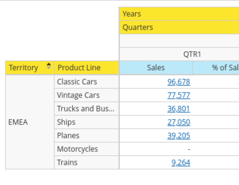
3. Drill through to the supporting data, in the analysis details, click the value for EMEA, Classic Cars, 2003, QTR1 ($96,678).

<figure><img src="/files/v80BZkuwBERec8BjqSqo" alt=""><figcaption><p>Drill-through - Classic Cars</p></figcaption></figure>
{% endtab %}

{% tab title="Formatting" %}
{% hint style="info" %}
You can resize columns, change the column or row header, and change data format.

To resize columns, click between the column headers and drag the resize icon to the left or right. You can reset all column sizes by clicking More > Reset Column Sizes from the Interactive Toolbar.

To change the column or row header for text and time period fields, right-click the column or row header and then select Edit

To format numeric data, right-click the column header and select Column Name and Format.
{% endhint %}

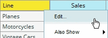
1. Right-click the column header for Line, then select Edit.

<figure><img src="/files/FnCCxtavZQtwgcgg2hdc" alt="" width="272"><figcaption></figcaption></figure>

2. In the Name text box, type Product Line, and then click OK.

<figure><img src="/files/aMsm5LHZTiIa0qlL8qOT" alt="" width="375"><figcaption><p>Edit header cells</p></figcaption></figure>

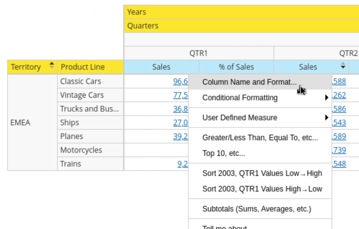
3. To modify the Sales data as currency, in the analysis details, right-click one of the Sales headers, then select Column Name and Format.

<figure><img src="/files/xrqrZWw1j7dOTpXMUtjx" alt="" width="563"><figcaption><p>Format Column</p></figcaption></figure>

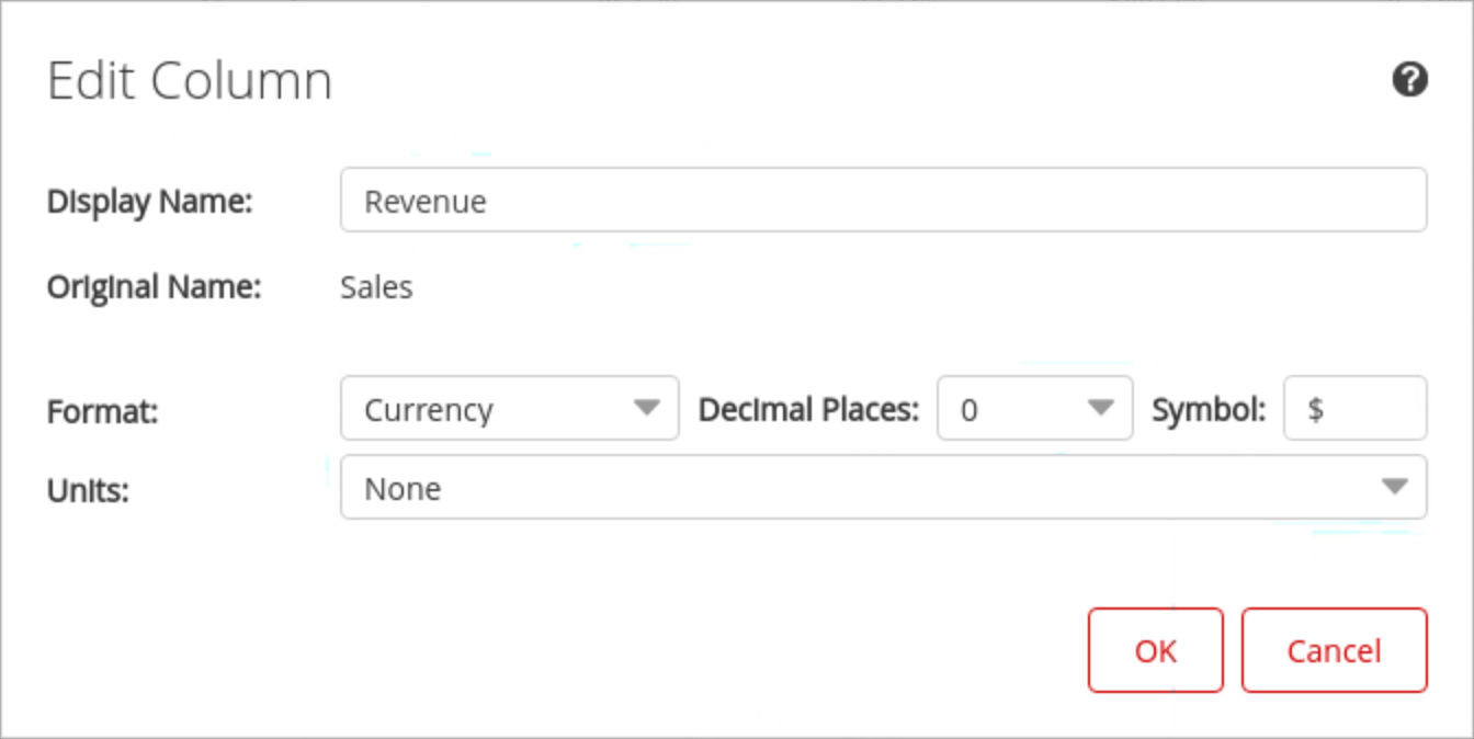
4. Change the name: Revenue

<figure><img src="/files/cFTTvKImIFSX0WonfNrv" alt=""><figcaption></figcaption></figure>

5. From the Format drop-down list, select Currency ($), and then click OK.

<figure><img src="/files/lsK1pVAckfdTxQrwKbHr" alt=""><figcaption><p>Formatting</p></figcaption></figure>

***

#### Chart Options

{% hint style="info" %}
At any point in time, an analysis can have only one format; however, it is easy to switch between formats.
{% endhint %}

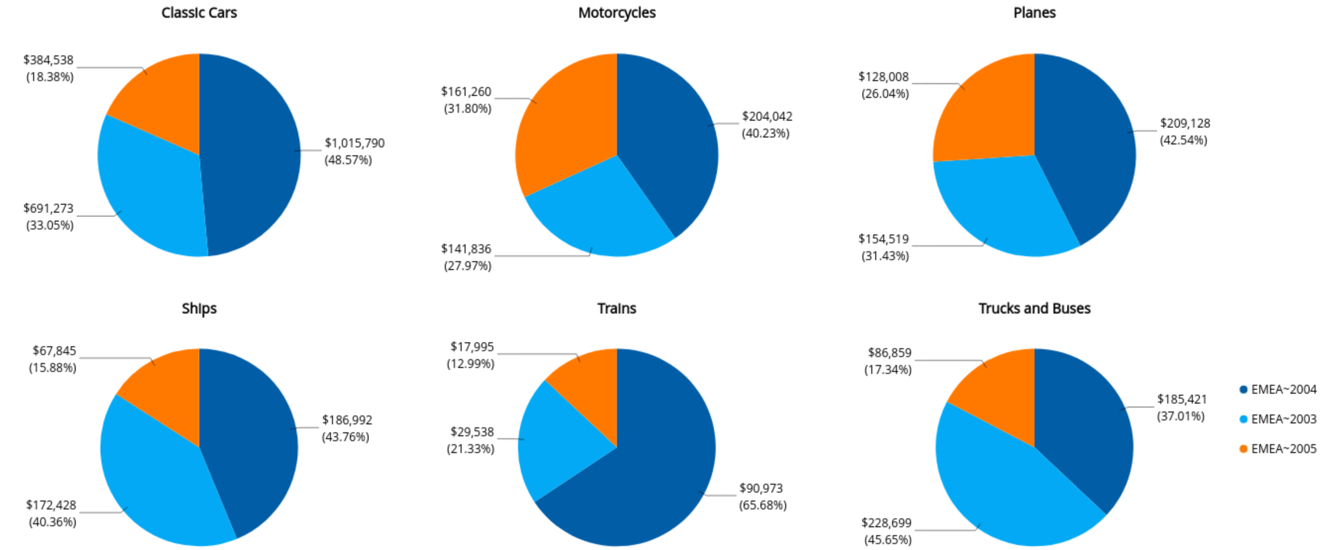
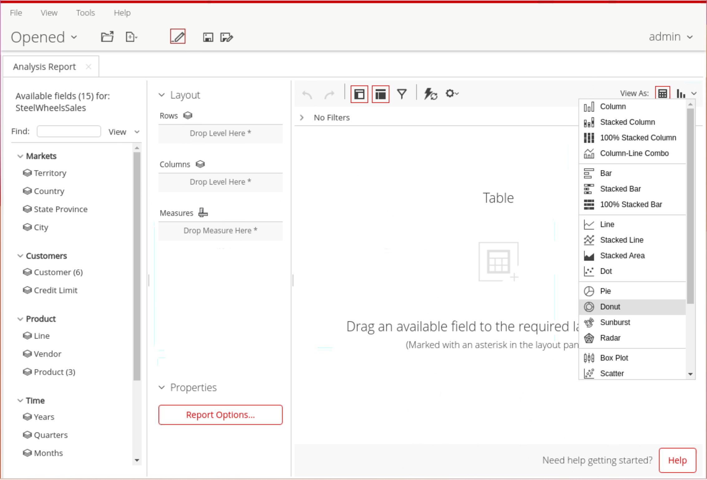
1. To switch the analysis format, click the View As Table or View As Chart button in the analysis title bar.

<figure><img src="/files/NbA5JcKxSng4wS7aShXM" alt=""><figcaption><p>Pie Charts for each Product Line</p></figcaption></figure>
{% endtab %}
{% endtabs %}
{% endtab %}

{% tab title="Actions & Options" %}
{% hint style="info" %}

#### Actions & Options&#x20;

{% endhint %}

<figure><img src="/files/DktytVsjCRXBZIwFGQD9" alt="" width="323"><figcaption><p>Actions &#x26; Options</p></figcaption></figure>

{% tabs %}
{% tab title="Export" %}
{% hint style="info" %}

#### Export Options

Analyzer provides several options for exporting your analysis. You can export the analysis as a PDF file which launches the analysis in a new window. From there you can save or print the PDF file. You can export the analysis to Excel, which opens the analysis in a new Excel window.

You can download the analysis data in CSV format. When you download data in the CSV format you get numbers with the full precision available. This way you avoid any rounding errors when you continue to work with your data in Excel. The export options are available from the Interactive Toolbar by clicking the More actions and options button.
{% endhint %}

<figure><img src="/files/QkmhU45nARNg0E1LGZZt" alt=""><figcaption><p>Export options</p></figcaption></figure>
{% endtab %}

{% tab title="Report Options" %}
{% hint style="info" %}

#### Report Options

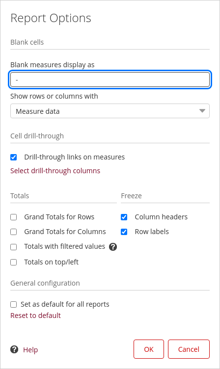
In your report, you can modify how blank measures display, define drill-through columns, and show or hide totals for columns and rows.
{% endhint %}

1. Click on the 'cog-wheel'.
2. Select: Report Options.

<figure><img src="/files/PFogKZIlwVHWf9Ozyr1v" alt=""><figcaption><p>Report Options</p></figcaption></figure>

{% hint style="info" %}
You can control what to show when a cell contains a blank value in your Analyzer report. Analyzer reports are designed to break down number fields, such as 'Sales', by text fields such as 'Product Name'.&#x20;

If a product did not sell, it will appear either as zero dollars or as a blank or a dash ("-"). In some reporting situations, the absence of a value could mean the same as a zero, but in other cases, zero might have a different meaning.&#x20;

The report calculations in the background behave differently depending on whether a value is 'blank' or a 'zero'. For example, when the report calculates averages, zeroes are considered whereas blanks are not.
{% endhint %}
{% endtab %}

{% tab title="Chart Options" %}
{% hint style="info" %}

#### Chart Options

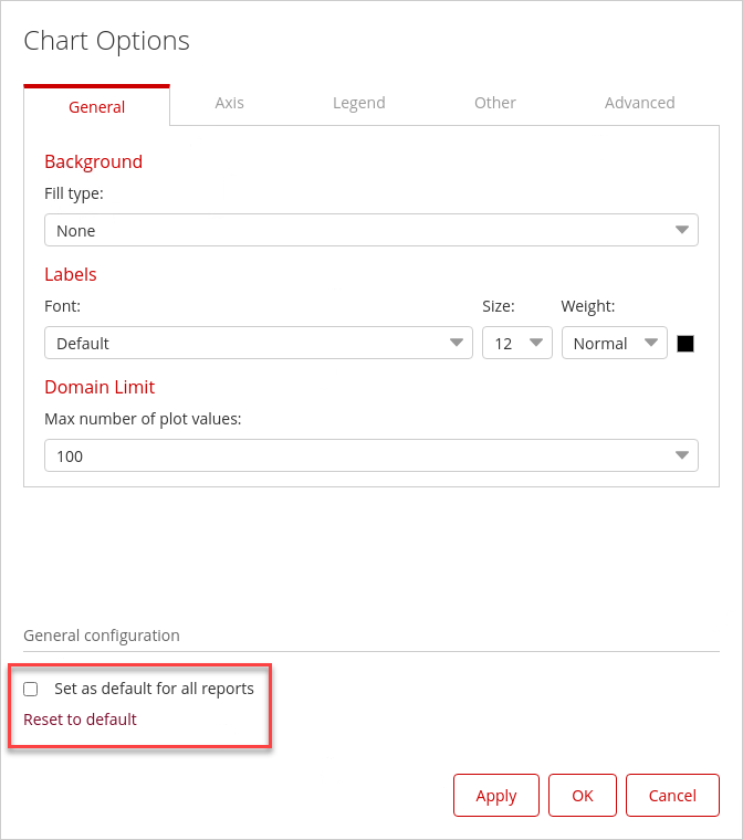
As an administrator, you can add default chart options that are applied whenever a new chart is created. Adding default chart options does not apply the changes to existing charts.&#x20;

You can modify the options on charts without affecting the default option settings.&#x20;

You can also set an existing chart back to the default settings by clicking the Reset to default link on the Other tab of the Chart Options dialog box.
{% endhint %}

1. Click on the 'cog-wheel'.
2. Select: Chart Options.

<figure><img src="/files/KntDahVJwemXVLx9Rhfo" alt=""><figcaption><p>Chart Options</p></figcaption></figure>
{% endtab %}

{% tab title="Administration" %}
{% hint style="info" %}

#### Adminstration

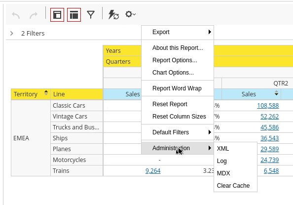
If been assigned the Administrator role, then you'll have access to some options that will help troubleshoot and optimize your PAZ reports.
{% endhint %}

1. Click on the 'cog-wheel'.
2. Select: Chart Options.

<figure><img src="/files/OgJRPIwe7WaDZ36Yo9Ne" alt=""><figcaption><p>Administration options</p></figcaption></figure>

***

{% hint style="info" %}

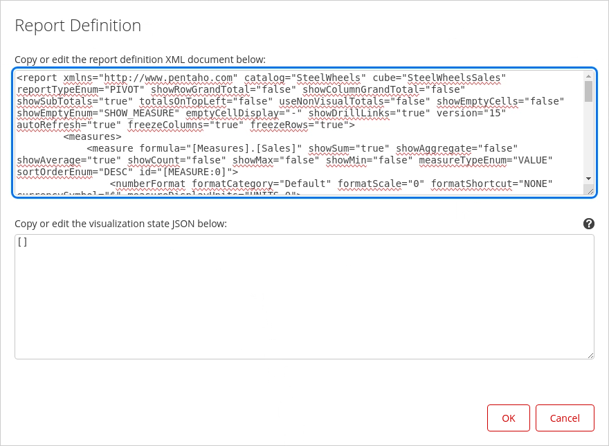
#### XML

Administrators can configure the default value of non-standard properties of the current visualization, at the report-level. This is useful for properties that are hidden from the user interface using a global configuration.

To perform this configuration, set the corresponding JSON text in the field Visualization state JSON, in the Report Definition dialog (Administration » XML).

For example, the following JSON configuration would change the colors used by many of the standard visualizations, by changing the value of the palette property:

\[ { "palette": {"colors": \["red", "green", "blue"]} } ]
{% endhint %}

<figure><img src="/files/f9uJZPx7mdLM4be3qvUF" alt=""><figcaption></figcaption></figure>

***

{% hint style="info" %}

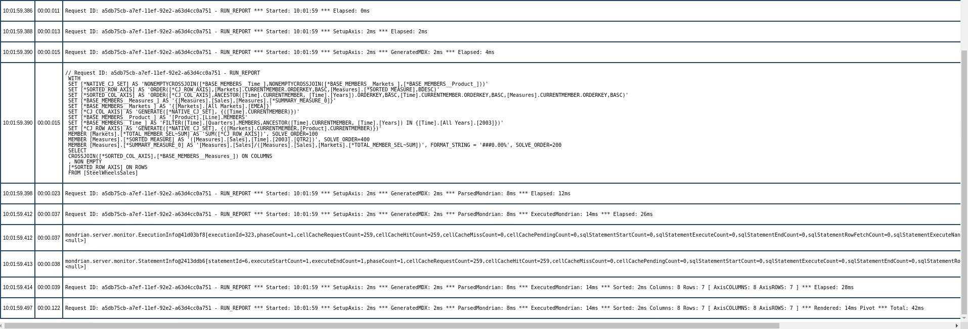
#### Log

Log option is useful for troubleshooting and optimizing your Analyzer reports. The first half of the log displays the xml of the report definition.

The second half display the MDX query and the times taken to execute the query.
{% endhint %}

<figure><img src="/files/mW7BUBG43nb384aMxRrZ" alt=""><figcaption><p>Log</p></figcaption></figure>

***

{% hint style="info" %}

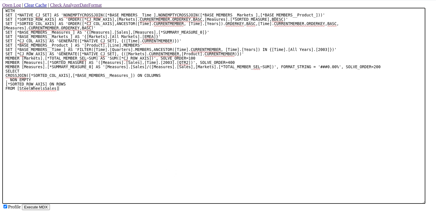
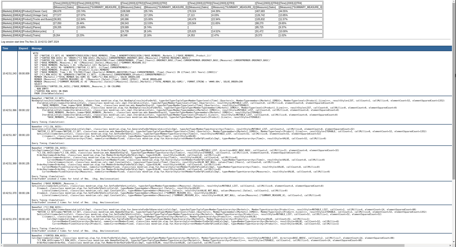
#### MDX

From here you're able to open the log file, Clear the Cache, Check the Time dimension and Execute MDX queries.
{% endhint %}

<figure><img src="/files/LY5zQWqWAVqtySNd5pgo" alt=""><figcaption><p>MDX</p></figcaption></figure>

<figure><img src="/files/6tzER9z1xSVsJvL1zIaD" alt=""><figcaption><p>MDX - output</p></figcaption></figure>
{% endtab %}
{% endtabs %}
{% endtab %}
{% endtabs %}


---

# Agent Instructions: Querying This Documentation

If you need additional information that is not directly available in this page, you can query the documentation dynamically by asking a question.

Perform an HTTP GET request on the current page URL with the `ask` query parameter:

```
GET https://academy.pentaho.com/pentaho-business-analytics/business-analytics/analyzer-reports/sales-analysis.md?ask=<question>
```

The question should be specific, self-contained, and written in natural language.
The response will contain a direct answer to the question and relevant excerpts and sources from the documentation.

Use this mechanism when the answer is not explicitly present in the current page, you need clarification or additional context, or you want to retrieve related documentation sections.